Machine and deep learning performance in out-of-distribution regressions

1. Introduction

Achieving a high level of performance in regression and classification tasks through machine learning (ML) and deep learning (DL) models poses a fundamental computational challenge, crucial for applications across diverse scientific and engineering fields [1–5]. The effectiveness of ML-based models is contingent on diverse components governing its performance such as the nature of the problem and the available data used to train the model [6–14]. A growing body of scholarship investigates the characteristics of a dataset in data-driven tasks in multiple aspects such as noise [15, 16], concept drift [17], and out of distribution (OOD) [18, 19].

The phenomenon of OOD data and its impact on data-driven (i.g., ML and DL) models has been the subject of extensive investigation due to its frequent occurrence and its challenging nature that causes unexpected complications in ML applications [20–22]. To illustrate the challenge posed by OOD scenarios, let us consider the example of a bike rental company that relies on a data-driven model to predict bike rentals based on past data. For years, the business was only open in nice weather, and the model trained and used on these days—provided highly satisfying results. However, recently, the business owner decided to extend the working days to the hot summer days as well. Unfortunately, the business’s model performing badly, causing a lot of economic harm. A possible explanation for the model’s poor performance on the summer days is that the hot summer days show different dynamics due to factors that are not necessarily taken into consideration in the original modeling and development. Hence, resulting in OOD data that the model fails to ‘understand’. To this end, understanding and addressing the challenges posed by OOD scenarios are critical for ensuring the robustness and reliability of data-driven models across diverse applications [23, 24]. Formally, OOD refers to data instances that deviate significantly from the training data distribution of data-driven models. This definition should be taken with caution as one should be careful not to confuse OOD with the concept drift phenomenon which describes the case where the data changes over time. OOD is a fundamental issue in data-driven modeling as it reveals the weakness of data-driven models which are designed to assume that the training data they provided is ‘well-representing’ the dynamics of the task [25]. Nonetheless, as illustrated by the above example, this condition is strenuous (or even impossible) to satisfy in many practical scenarios.

In order to address this challenge, in this study, we present a novel usage of the well-established symbolic regression (SR) method as a tool to improve ML and DL model’s extrapolation capabilities, making them more robust in terms of OOD. SR is a computational technique used in ML and evolutionary algorithms to automatically discover mathematical expressions that best fit a given dataset [26–28]. Intuitively, SR models have been shown to be less expressive and accurate than ML and DL models when considering in-distribution (ID) performance (i.e. the distribution defined by the training data proposed to the data-driven model) [29, 30]. The so-called ‘under-representation’ of SR models often also results in their ability to capture the main dynamics behind a sampled dataset and therefore has the potential to generalize better for OOD samples [31–33]. By incorporating SR-derived features before applying ML and DL models, we show that ML and DL perform (statistically) similarly (or even better) on in-distributing evaluation while also outperforming OOD evaluation.

We evaluate the proposed method by applying two ‘off-the-shelf’ SR models (QLattice [34] and GPlearn [35], automatic ML Tree-based Pipeline Optimization Tool (TPOT [36]), and automatic DL models (AutoKeras (AK) [37]) on n = 15 real-world datasets from various domains and with various properties. Our analysis shows that the ML and DL performance for the ID evaluation improved by a mean of 2.85% and 11.05% (p < 0.01), respectively, compared to the same models without the SR enhancement. As for the OOD data, the inclusion of the SR-derived feature improved the performance of the ML and DL models by a mean of 3.70% and 10.20% (p < 0.01), respectively.

The remainder of this paper is organized as follows: section 2 provides an overview of related work in the field of OOD, discussing various definitions of OOD and current solutions as well as SR methods with their strengths and limitations. Afterward, section 3 presents our proposed method that includes the data used in the experiments, the SR as a tool to tackle OOD, and the experiment design conducted in this study. Next, section 4 outlines the obtained outcomes. Finally, in section 5, we discuss the implications and possible applications drawn from our results while also discussing the limitations of the study and promising future work.

2. Related work

OOD is a commonly found challenge of data-driven models, in general, and for ML and DL models, in particular, [38–40]. In parallel, SR has been shown as a powerful computational tool that has palatial generalization capabilities for tabular data [41]. In this section, we provide an overview of existing solutions for OOD in ML and DL settings. Subsequently, we provide an overview of SR methods with a focus on their potential as an extrapolator that can be utilized for the OOD challenge.

2.1. Out of distribution in data-driven models

The fundamental premise of data-driven models, in general, and in ML (and DL) models, in particular, is based on the assumption that data will be identically and independently distributed (i.i.d). This means that the training and test data are assumed to come from the same distribution. This assumption often fails to hold in numerous real-world scenarios [42]. In recent years, ML and DL algorithms have become ubiquitous across various domains of life and their usage ‘outside of the lab’, when deployed in real-world settings, often encounter violations of the closed-world and i.i.d assumptions [43–45]. This decline in performance is typically attributed to shifts in data distributions [46]. Currently, there is an active investigation of this phenomenon, commonly referred to ‘OOD’ [47, 48]. A few recent studies have tackled this challenge and estimated the OOD degradation in different datasets [49, 50].

In addressing OOD scenarios within ML and DL, various solutions have been explored [51]. For instance, [52] builds on top of the Risk Extrapolation mathematical framework, as a form of robust optimization over a perturbation set of extrapolated domains, to show that reducing differences in risk across training domains can reduce a model’s sensitivity to a wide range of extreme distributional shifts. Yao et al [53] proposed a simple mixup-based technique that learns invariant predictors via selective augmentation called LISA. Simply put, this method selectively interpolates samples either with the same labels but different domains or with the same domain but different labels in the case of subpopulation shifts (e.g. imbalanced data) and domain shifts. Moreover, [54] extended the task of improving the robustness to OOD by combining an OOD detection mechanism as an inherent part of the method. Namely, the authors propose a margin-based learning framework that exploits freely available unlabeled data in the wild that captures the environmental test-time OOD distributions under both covariate and semantic shifts. Taken jointly, [55] empirically showed that OOD performance is strongly correlated with ID performance for a wide range of models and distribution shifts. In particular, the authors connected the power of this connection to the Gaussian data model revealing that the further a sample from the center of the Gaussian’s defined centroid, the weaker the connection is.

Despite these advancements, challenges persist in effectively addressing OOD in data-driven models. Evaluating OOD detection methods remains a complex task due to the inherent imbalance between ID and OOD samples. Additionally, while existing techniques provide valuable insights, understanding the implications of OOD data in specific application domains, such as medical imaging, autonomous systems, and natural language processing, remains an ongoing area of research. Further advancements are needed to enhance the robustness of models in the presence of OOD data, especially in diverse and complex real-world scenarios.

2.2. Sr

SR can be addressed through diverse techniques, including brute-force search, sparse regression, DL, and genetic algorithms [56, 57]. While each method has its strengths and weaknesses, no single approach dominates the field [27].

Initially, brute-force SR models theoretically have the potential to solve any SR task by exhaustively evaluating all possible equations to find the optimal one [58]. However, in practice, applying brute-force methods often becomes impractical due to the significant computational demands, making them challenging to use even with relatively small datasets. Moreover, these models tend to overfit when dealing with large and noisy data [59], which is frequently encountered in real-world scenarios [60]. In contrast, DL SR models excel at handling noisy data, thanks to the inherent robustness of neural networks against outliers [61]. Nevertheless, empirical evidence suggests that these models have limited generalization capabilities, which restricts their applicability in many contexts [27, 62]. Sparse regression methods have gained popularity by significantly narrowing the search space through sparsity-driven optimization, enabling the discovery of concise models [63]. For example, SINDy [64] employs a Lasso linear model to uncover sparse representations of nonlinear dynamical systems underlying time-series data. The algorithm alternates between a partial least-squares fit and a thresholding step to encourage sparsity. Due to the potential of this method across various domains, it has garnered significant attention, with researchers enhancing its performance by introducing mechanisms to better handle noisy data and select optimal models across varying threshold values [65–67]. Finally, genetic algorithm SR models effectively integrate prior knowledge to constrain the function search space [68]. For instance, SR can be guided by predefined solution shapes [69–72], or by probabilistic models that sample grammar rules governing solution generation [73–77].

SR is known to overfit data less than more complex ML or DL models [30], indicating a greater potential for generalization and OOD performance. SR has been demonstrated to outperform other ML models on small datasets [30]. The concept of ‘under-representation’ in SR models often allows them to capture the primary dynamics of a sampled dataset, potentially improving their ability to generalize to OOD samples [31–33].

3. Methods and materials

3.1. Dataset

We performed the analyses on a benchmark of regression datasets from a recent benchmarking study on automatic ML regression tasks [78]. Specifically, we analyzed a total of 15 datasets from seven studies [79–85]. The only modification we applied to the datasets was the removal of categorical variables, as we focus exclusively on numerical variables since classical SR does not support categorical variables. This modification does not influence the results as these are relative to each other.

3.2. Experimental setup

We examine the ID versus OOD performance of different ML and DL models, under different definitions of OOD. To ensure the robustness of our results, we perform 50 repetitions of the experiment for each of the 15 datasets and for each of the ML or DL models.

In each iteration of each dataset, we begin by splitting the data into ID and OOD using a given OOD metric. We define OOD observations as the 15% highest OOD-metric observations, for a given OOD measure. We then split the ID data into 70% training, 15% validation data, and 15% test data. We then train an ML or DL model on the training data and evaluate its root mean squared error (RMSE) performance on both the ID test data and the OOD data.

We adopted four popular OOD definitions from those proposed in [48]. First, we use the multivariate Z-score. Formally, in the univariate case, the Z-score of an observation from the mean of a univariate normal distribution is derived by taking the mean and standard deviation of one of the input features. For example, a Z-score of 0 would indicate an observation that is equal to the mean score, and a Z-score of 1 would indicate that the observation is one standard deviation away from the mean. The multivariate generalization of the Z-score was first introduced by Mahalanobis in 1936 [86] and is referred to as the Mahalanobis distance. Considering a probability distribution Q over R^N, characterized by its mean vector⃗µ = (µ₁,µ₂,µ₃,...,µ_N)^T and a positive-definite covariance matrix S, the Mahalanobis distance d_M from a point x = (x₁,x₂,x₃,...,x_N)^T to Q is defined as:

In the univariate case, the Mahalanobis distance is identical to the Z-score. This definition of multivariate Z-score has been widely used and is probably the most common definition for OOD in regression tasks [87–95]. Second, as a robustness test, we consider a random-feature Z-score. For this case, we randomly (in a uniformly distributed manner) choose one feature in each iteration and define the observation as either in or out of distribution based on its Z-score [96]. Third, as an additional robustness test, we also use a weighted distance inspired by the Kullback–Leibler (KL) divergence metric. KL divergence is a concept from information theory used to measure how one probability distribution diverges from a second, reference probability distribution. In the context of OOD, KL divergence is utilized to quantify the difference between the probability distributions of ID and OOD data [97]. Finally, we use an OOD metric based on the y-sparsity, as performed in the novel work of [49].

3.3. ML and DL models

For the experiment, we adopted several popular ML and DL methods, ranging from the simplest one linear regression (LR) to more advanced models (AK):

• • TPOT [36]—an automated ML tool that uses genetic algorithms [98] to optimize ML pipelines, including data preprocessing, feature selection, and model selection. As an AutoML library, TPOT performs hyperparameter optimization intrinsically. The only limitation we used was a time limit of 10 min per individual fold run. Time limited model runs are common in tabular benchmarks to ensure a fair comparison between different models [99–101].
• • AK [37]—an open-source automated ML library built on top of Keras, which automatically searches for the best neural network architecture and hyperparameters for a given dataset. Similar to TPOT, AK performs hyperparameter optimization intrinsically. We limited its runs to at most 200 epochs.
• • XGBoost (XGB) [102]—an optimized gradient boosting algorithm that is highly efficient and widely used for classification and regression tasks, known for its performance and scalability. Hyperparameter optimization was performed using TPOT, with a 10 min time limit per run.
• • Random forest (RF) [103]—an ensemble learning method that constructs a multitude of decision trees [104] during training and outputs the mode of the classes or mean prediction of the individual trees for classification or regression tasks, respectively. Hyperparameter optimization was performed using TPOT, with a 10 min time limit per run.
• • Support vector machine (SVM) [105]—a supervised ML algorithm used for classification and regression tasks, which finds the hyperplane that best separates classes in a high-dimensional space. Hyperparameter optimization was performed using TPOT, with a 10 min time limit per run.
• • K-nearest neighbors (KNNs) [106]—a non-parametric, instance-based learning algorithm used for classification and regression tasks, where the classification of a data point is determined by a majority vote of its KNNs in the feature space. Hyperparameter optimization was performed using TPOT, with a 10 min time limit per run.
• • LR [107]—a statistical method used for modeling the relationship between a dependent variable and one or more independent variables by fitting a linear equation to the observed data.

3.4. Integration of SR in ML and DL models

We use the method proposed by [108] to examine a method to improve OOD performance. Namely, The authors propose using SR as a feature engineering technique to enhance ML and DL regression models. Through extensive experiments on synthetic and real-world datasets, they demonstrate that incorporating SR-derived features significantly improves model performance, with gains in RMSE of up to 11.5% on real-world datasets. The study highlights the potential of SR for improving model accuracy and interpretability while reducing the reliance on domain expertise for feature design. In this work, we extend the investigation of this method by exploring the SR-derived feature contribution to ID and OOD separately, rather than the entire dataset at once. We hypothesize that due to the SR’s tendency not to overfit the data, its contribution to ML or DL OOD performance might be even higher compared to ID performance. To examine this hypothesis, we repeat the experiment described in section 3.2 either with or without an SR-derived feature, for both TPOT and AK. AK is used as a model which estimates various DL architechtures, while TPOT evaluates various ML models, including those mentioned above (XGB, RF, KNN, and SVM). We use two different SR models to establish the robustness of this method. First, GPlearn [35] which is a popular open-source Python library that uses genetic algorithms to fit expression trees over provided data such that the expression tree’s prediction is as close to the predicted parameter while also the expression’s complexity is minimal. Second, QLATTICE [34] which is an open-source Python library that searches for expression trees containing only multiply, linear, sine, tanh, and gaussian (unlike the other two libraries that used addition, multiplication, division, subtraction, and inversion). This library first ‘guesses’ the structure of the expression tree followed by a training procedure which both allocates the right expressions to the tree and the weights of their inputs. It uses a genetic algorithm to search over the expression tree structures.

In the GPlearn model, we utilized the four basic operators: addition, subtraction, multiplication, and division. Additionally, we conducted 200 trials using the default operators in GPlearn, finding no significant variations (results not shown). The modeling was carried out over 50 generations, with the model being tested six times using various parsimony coefficients (0.005, 0.01, 0.02, 0.03, 0.04, 0.05). For each test, the parsimony coefficient that yielded the lowest RMSE on the training data was chosen. Other than these hyperparameters, we maintained all other settings at GPlearn’s default values. In the Feyn model we evaluated various complexity values (5, 10, 15, 20, 25, 30) and chose the highest performing value. Other than that, we used the default hyperparameters of the library.

4. Results

In this section, we present the results of the experiments. First, we outline the performances of various ML and DL models in ID compared to OOD scenarios. Afterwards, we examine the integration of SR-derived features into the performance of ML and DL models in ID and OOD scenarios.

4.1. ML and DL performance in OOD data

Figure 1 presents an example of the results in a single dataset. In this example, Z-scores are determined based on the temperature variable. The target feature, hourly bike rentals, is predicted by the XGB model trained on ID data and tested on both ID and OOD observations. The horizontal axis represents the Z-score and the vertical axis represents RMSE for each observation. As expected, RMSE performance is best for lower Z-scores and deteriorates for higher Z-scores.

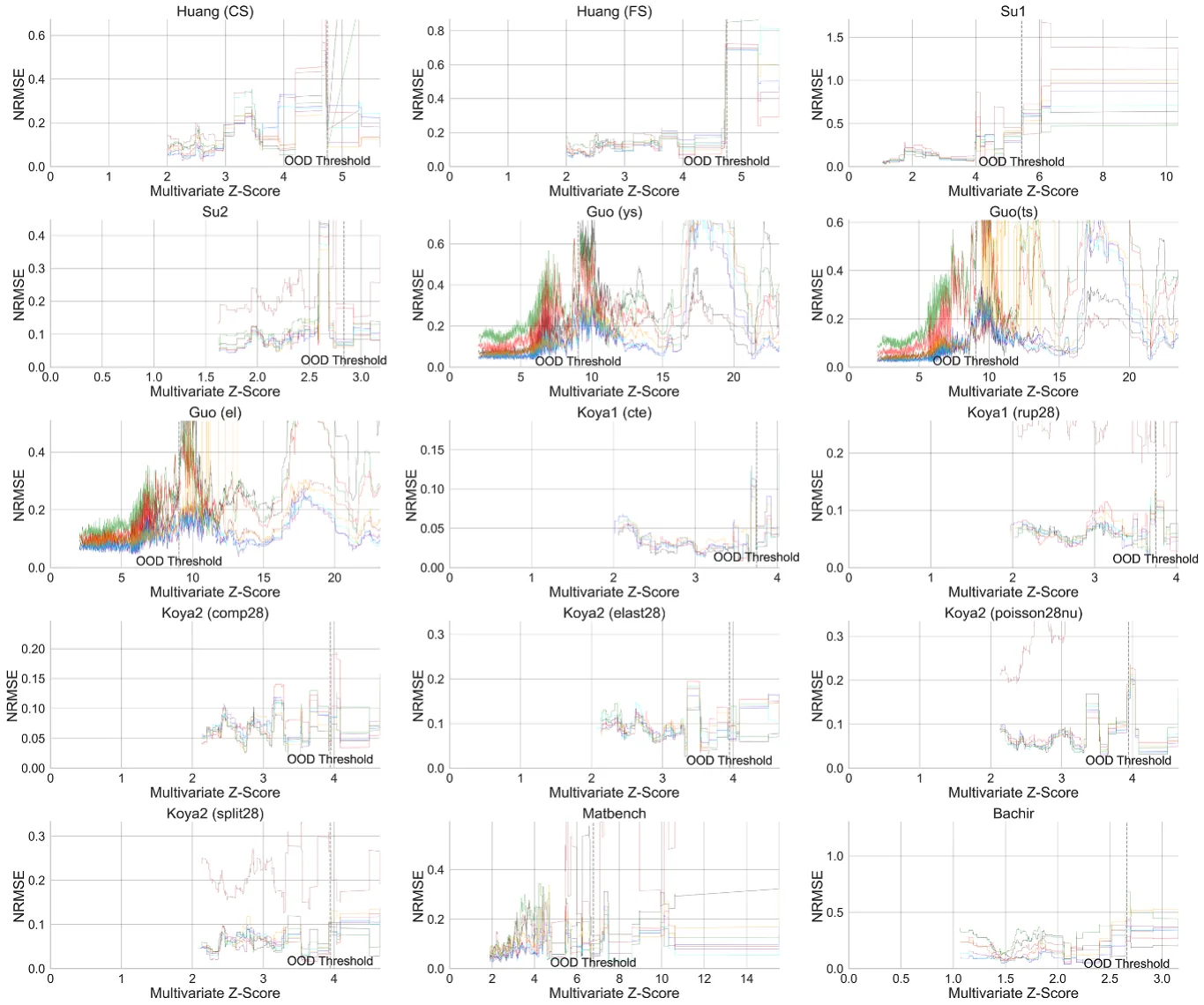
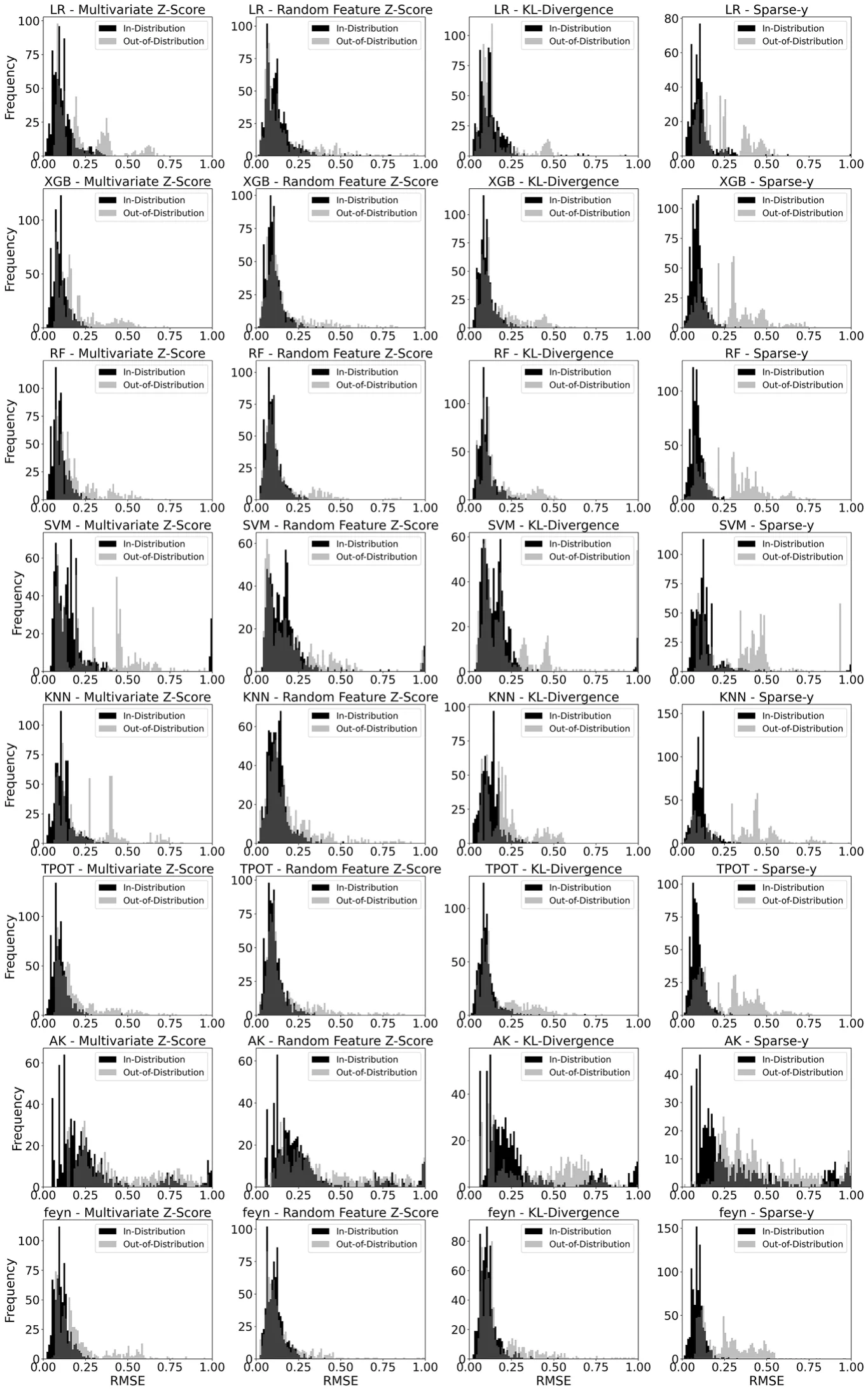
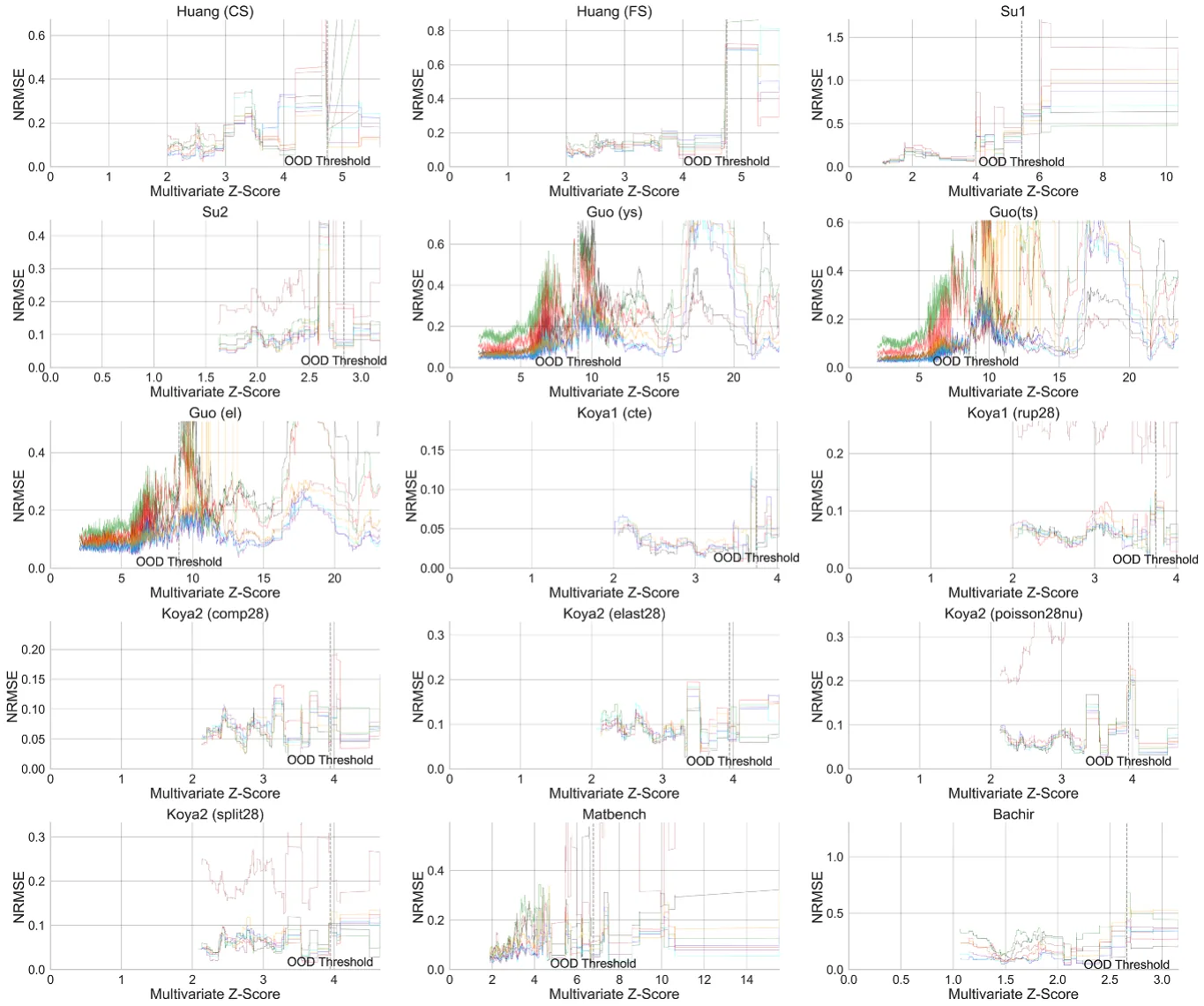
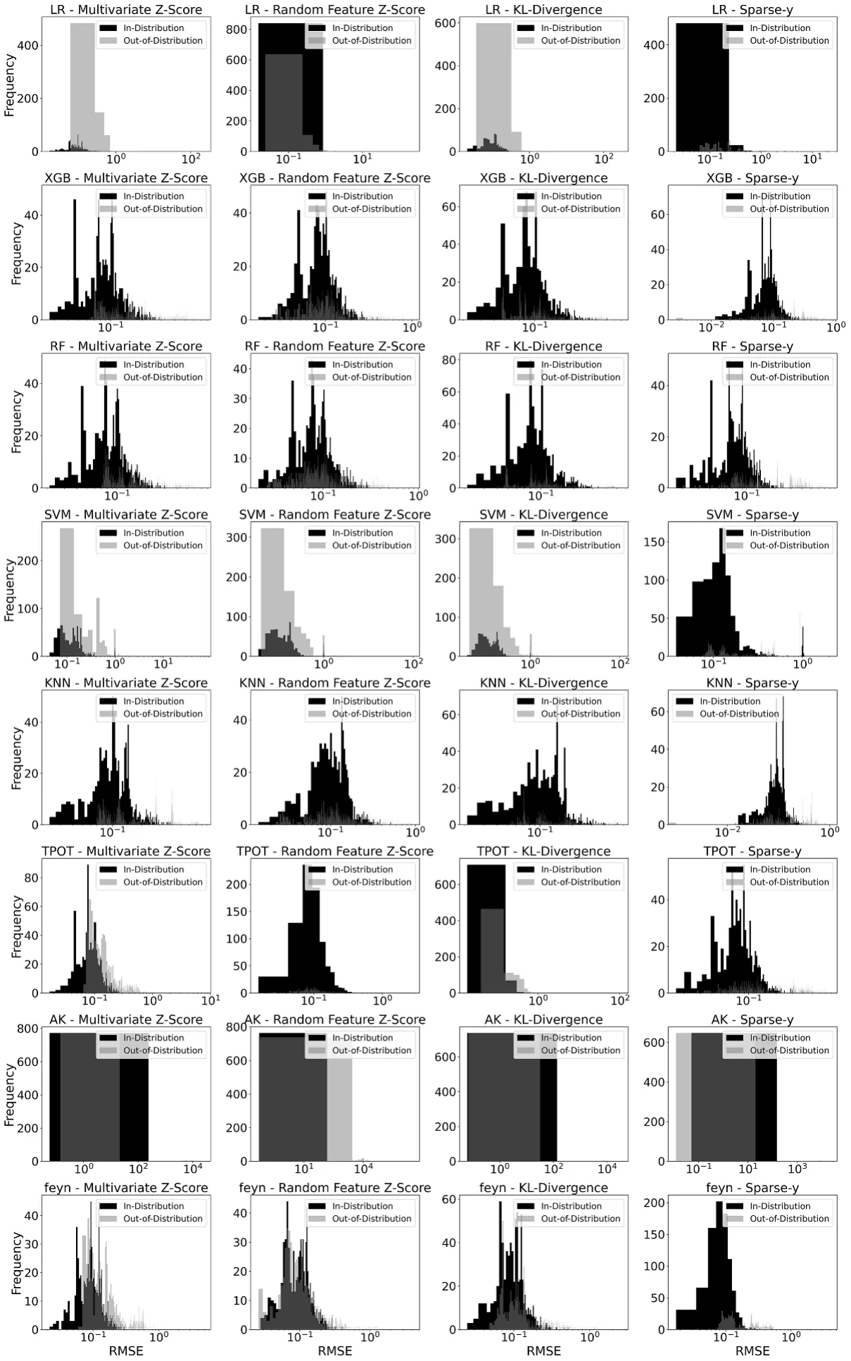
Figure 2 and table 1 present a complementary analysis for the entire benchmark of 15 datasets. Figure 2 uses multivariate Z-score as an OOD metric; additional metrics are presented in the appendix. To present datasets of different scales in one figure, we normalize the RMSE scores by dividing them by the corresponding dataset’s mean absolute y (target feature) value. Figure 3 presents the histograms of ID and OOD errors in each model and OOD metric. The results of our experiments reveal several intriguing patterns. Firstly, we observed that the performance of various ML and DL models, including XGB, RF, and TPOT, tends to degrade as the Z-score increases, indicating a decline in model accuracy for OOD data. Table 1 provides both the difference (%) between OOD and ID data, and the slope of a LR in the RMSE versus OOD figures. Both the difference and the slope are always positive, demonstrating the robustness of this result. This finding is consistent with the expected behavior of ML models when encountering data that deviate significantly from the training distribution.

Interestingly, while all models experienced a decrease in performance for OOD samples, the extent of this degradation varied across different models. For instance, RF demonstrated a relatively better resilience to OOD data compared to other models, including XGB. This could be attributed to the inherent robustness of ensemble methods like RF, which combine predictions from multiple decision trees to reduce variance and improve generalization.

Another noteworthy observation is the similarity in the shape of the RMSE versus Z-score curves across different models, albeit with varying magnitudes of RMSE. This suggests that certain OOD samples pose a consistent challenge to all models, regardless of their underlying algorithms. Identifying the characteristics of these particularly challenging OOD samples could provide valuable insights for designing more robust ML models. We also observe that the performance trend with respect to the Z-score is not monotonic, indicating that certain OOD observations are not as challenging to predict as others.

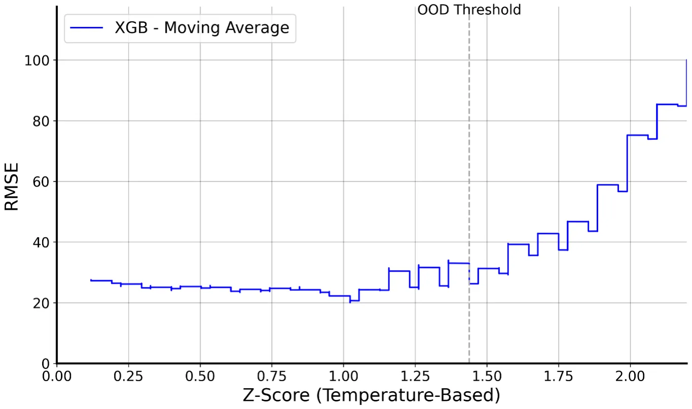
Figure 3 shows the difference between ID and OOD performance as histograms. While some OOD data align with the distribution of ID samples, the OOD errors generally exhibit a much larger tail, indicating that some OOD predictions had significantly larger errors. In some instances, the OOD errors extended beyond merely forming a tail; they were also centered around higher error values. This phenomenon could stem from the integration of multiple datasets, where, in certain datasets, OOD errors deviated markedly from ID errors and were centralized around higher error values.

Lastly, our findings reveal that although the AK model typically exhibited lesser performance compared to other ML models, in line with prior studies, it surpassed even the top-performing ML models in certain high OOD scenarios. This unexpected outcome merits further investigation.

4.2. Integration of SR in ML and DL models to improve OOD performance

In this section, we examine the contribution of integrating an SR-derived feature before the application of ML or DL models [108]. As demonstrated in figure 2, SR does not perform as well as other ML models (such as XGB and RF) in ID observations. However, its performance in OOD observations is only slightly inferior compared to these models, suggesting that features derived from SR could be beneficial for ML models in OOD scenarios.

In table 2 we further evaluate the robustness of this method using two different SR models, and four different measures of OOD. We find that the improvement in performance is robust and holds in all 24 configurations (two different SR models, three different OOD metrics, and two different ML and DL models, either in or out of distribution). Furthermore, in most cases (9 of 12) the relative improvement in OOD is larger than the relative improvement in ID, consistent with our hypothesis that the SR-derived feature contributes more in this type of data.

The integration of SR-derived features into ML and DL models further emphasizes the potential of SR as a tool for enhancing model performance in OOD scenarios. The improvement in both ID and OOD performance suggests that SR-derived features can capture underlying patterns in the data that are not easily detected by conventional ML models. This could be particularly useful in applications where interpretability and generalization to novel scenarios are crucial.

Overall, our results highlight the importance of considering OOD performance in the evaluation of ML models and suggest that incorporating SR-derived features can be an effective strategy to improve model performance, robustness, and interpretability.

OOD Type	Multivariate-Z		Random feature Z-score		KL-divergence		Sparse-y
Model	Diff (%)	Slope	Diff (%)	Slope	Diff (%)	Slope	Diff (%)	Slope
LR	145	0.025	49	0.026	41	0.000 239	110	0.10
XGB	69	0.013	33	0.016	47	0.000 140	173	0.16
RF	89	0.016	27	0.017	41	0.000 148	141	0.19
SVM	63	0.022	8	0.015	21	0.000 233	87	0.14
KNN	78	0.018	42	0.021	55	0.000 143	172	0.19
TPOT	77	0.014	38	0.013	36	0.000 206	139	0.15
AK	67	0.102	42	0.054	44	0.000 586	131	0.12
Feyn	85	0.020	41	0.021	49	0.000 118	144	0.12

5. Discussion

In this study, we explored the performances of various ML and DL models in regression task tests on both ID and OOD samples. To ensure the robustness of our results, we performed extensive modeling with various models (XGB, RF, KNN, SVM, LR, TPOT, AK, gplearn, QLattice), a relatively large benchmark of n = 15 real-world datasets, and multiple repetitions (n = 50 each), resulting in over 40000 model runs. We summarized our results by displaying and comparing the obtained RMSE values for each model as a function of multivariate Z-scores, random feature Z-score, and KL-Divergence.

Based on the obtained results, we found that XGB and RF are not only the best-performing models, but they also maintain a relatively high performance in OOD samples. Also, the DL models performed surprisingly well in OOD data, despite their relatively lower performance in ID data. This observation can be attributed to the DL models’ ability to transform the feature space effectively. Even when the original feature space suggests sparsity or outliers, these models can create a learned feature space where such sparse samples are denser, thus not as sparse in the transformed context. While the various models obtained substantially different RMSE scores in both ID and OOD samples, the shape of the RMSE versus Z-scores figure remained remarkably similar between all models, with different stretch factors in the vertical axis. As such, we conclude that some OOD samples are harder to predict than others, making it difficult for all models to perform well in their prediction. Finally, we note that this shape is not monotonous, meaning that in some cases there are samples that are harder to predict than others, although their OOD-metric is lower. This property raises a question about the current OOD definitions commonly used.

		TPOT
		Feyn	gplearn
OOD type	ID (%)	OOD (%)	ID (%)	OOD (%)
Multivariate Z-score	2.56	4.74	1.92	2.80
Random feature Z-score	3.15	4.60	2.74	5.22
KL-divergence	3.50	1.25	3.23	3.60
Sparse-y	3.22	3.22	5.59	1.92
		AK
		Feyn		gplearn
OOD type	ID (%)	OOD (%)	ID (%)	OOD (%)
Multivariate Z-score	14.32	10.34	8.89	9.82
Random feature Z-score	12.31	13.70	9.13	9.33
KL-divergence	12.42	4.71	9.30	13.14
Sparse-y	11.09	16.08	7.09	17.35

To improve the OOD performance of these models while preserving the ID performance, we have introduced a novel approach to predictions in OOD, based on the SR method. Namely, we add additional features to the models by solving an SR task between the input and target variables, before repeating the same task using the ML (DL) model. This outcome undeniably showcases the capacity of features derived from SR to markedly improve the OOD predictive performance of data-driven models. These results indisputably highlight how features obtained through SR have the potential to significantly enhance the predictive capabilities of data-driven models as these provide these models with a generalized yet under-representing representation of the data that these models can use to improve their generalization capabilities. Our analysis indicates that for ID evaluation, the performance of ML and DL models enhanced by a mean of 2.85% and 11.05%, respectively (p < 0.01), with the addition of the SR enchantment. Regarding the OOD data, incorporating the SR-derived feature resulted in a performance improvement of 3.70% and 10.20%, respectively, for ML and DL models (p < 0.01).

Moreover, as illustrated in table 2, the proposed SR method can statistically improve the OOD performance with different definitions of OOD. Furthermore, table 2 supports the fact that this outcome is preserved on a large number of datasets from different domains and diverse properties. As demonstrated from the table, the SR-derived feature improves the ML and DL models while the SR model by itself produces an inferior RMSE score on the same OOD samples. Thus, the combination of the two methods—SR and ML/DL, obtained the highest performance. In addition, the inclusion of SR-derived features can enhance the interpretability of ML models and help prevent overfitting.

While our study underscores the potential of combining SR and ML (DL) models to improve their OOD performance, there are several limitations to this study. First, the suitability of SR may differ based on dataset characteristics, prompting inquiries into its adaptability across diverse domains and the computational properties inherent in the dataset [26, 27]. Second, this study employed two SR methods - (QLattice [34] and GPlearn [35]). Further exploration of other SR models could yield slightly different results [27]. This raises the computational question of finding the best SR model based on dataset characteristics, and optimizing its effectiveness for the OOD task [7]. Finally, the study highlights the importance of estimating confidence intervals in ML models, especially in OOD predictions where larger estimation errors are expected.

Data availability statement

All data that support the findings of this study are included within the article (and any supplementary files).

Funding

This research did not receive any specific grant from funding agencies in the public, commercial, or not-for-profit sectors.

Appendix

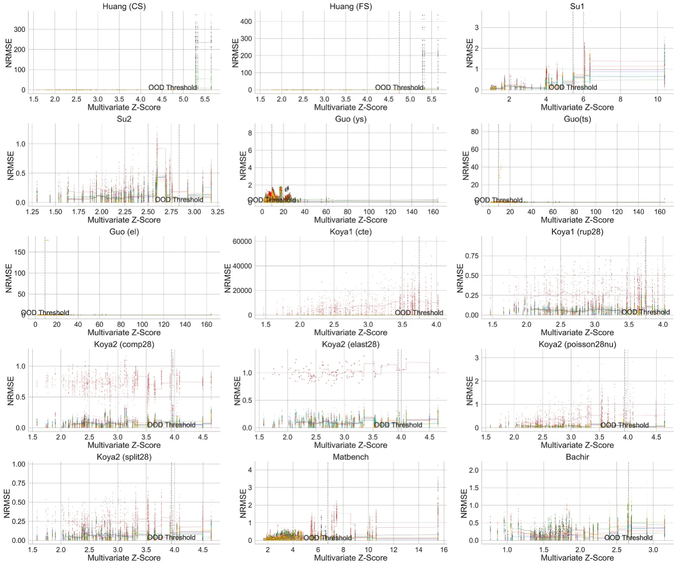
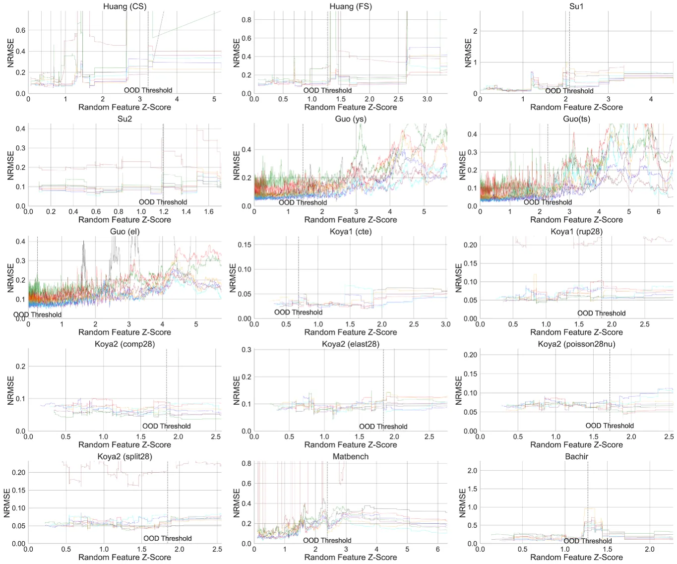
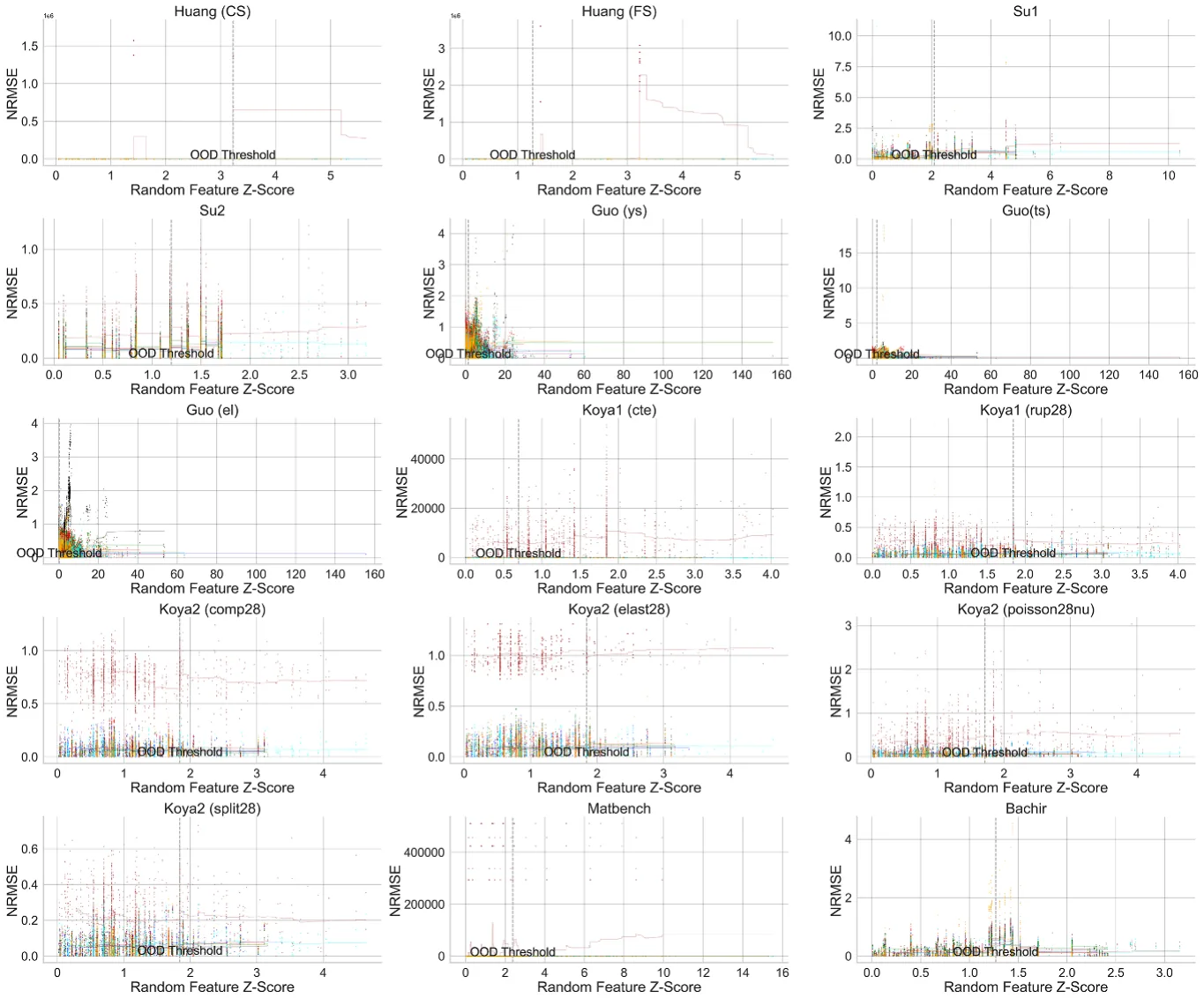
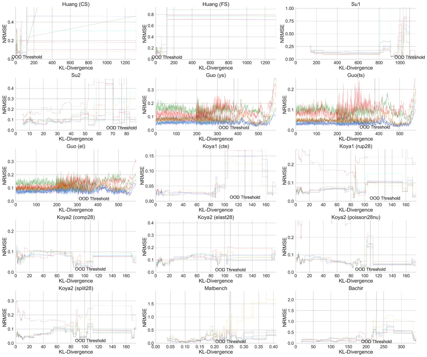
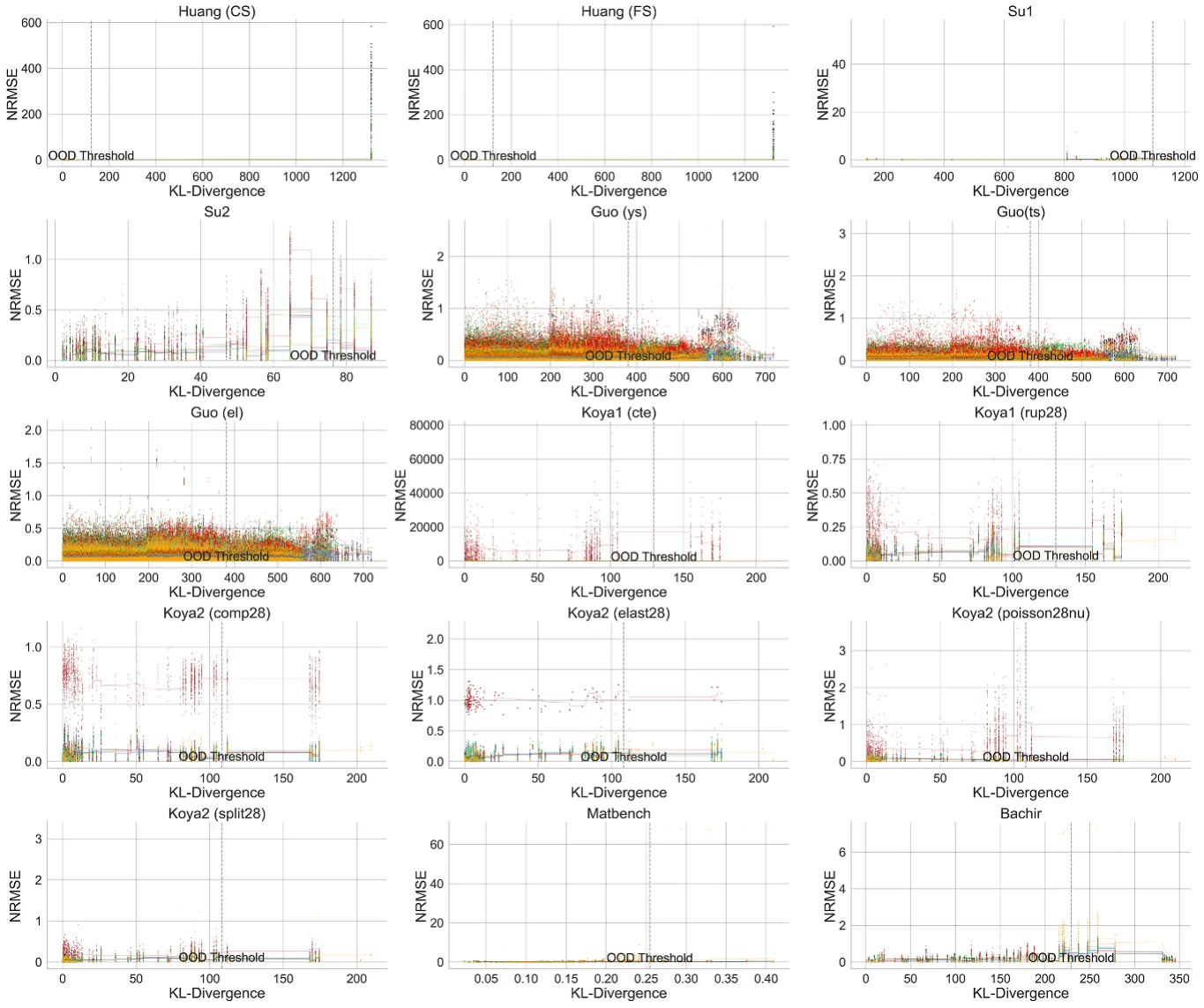
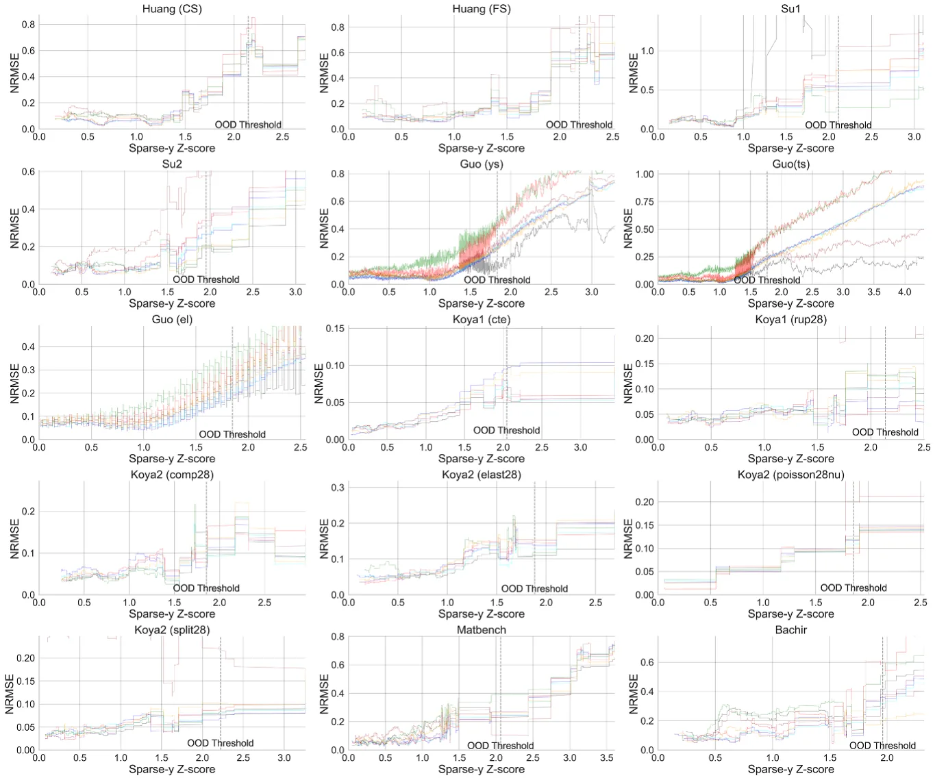
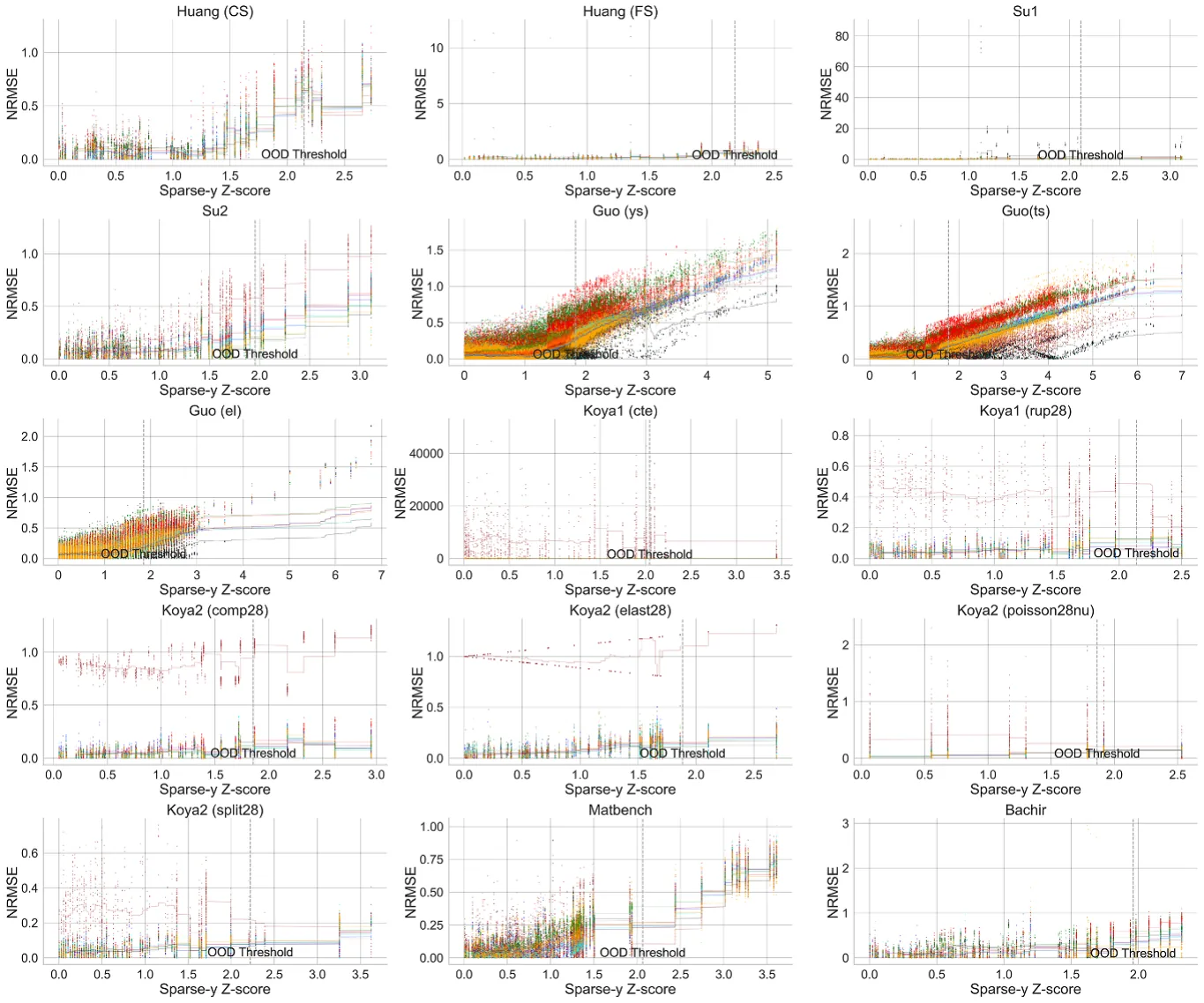
Table A.1 presents the descriptive statistics of the datasets used in the study. Figures A.1, A.3, A.5, and A.7 break down the information presented in figure 2 into separate datasets. Figures A.2, A.4, A.6, and A.8 do the same and present the entire range, including outliers. Tables A.2–A.5 summarize the results for the multivariate Z-score, random feature Z-score, KL-Divergence, and y-sparsity, respectively.

Dataset	# Rows	# Columns	# Categorical columns	Average feature entropy	Kurtosis
Matbench	312	23	0	9.2786	372.6246
Su 1	122	8	6	4.6943	3.1692
Su 2	136	6	5	4.8412	−1.3164
Koya 1 (Rup28)	110	11	8	4.6749	1951.502
Koya 1 (Cte)	110	11	8	6.4352	1420.308
Koya 2 (Split28)	110	11	7	8.9995	1160.730
Koya 2 (Poisson28nu)	110	11	8	8.1476	720.4195
Koya 2 (Elast28)	110	11	7	5.8595	1016.892
Koya 2 (Comp28)	110	11	7	9.7617	−2046.0
Huang (FS)	114	10	9	4.4699	3.1935
Huang (CS)	114	10	9	4.4656	3.1935
Guo 1 (Ys)	63 162	28	3	10.4080	861.2404
Guo 2 (Ts)	63 162	28	3	10.4088	861.2404
Guo 3 (El)	63 162	28	3	10.4089	861.2404
Bachir	112	4	2	4.6315	−0.6539

		LR				XGB
	ID	OOD	Diff (%)	Slope	ID	OOD	Diff (%)	Slope
Combined (mean)	—	—	9128	5.026	—	—	91	0.038
Combined (median)	—	—	145	0.025	—	—	69	0.013
Koya1 (rup28)	57.277	64.467	12.55	0.003	56.614	64.539	14.0	−0.0
Koya2 (comp28)	450.86	443.442	−1.65	0.01	543.184	496.164	−8.66	0.009
Koya2 (elast28)	467 825.449	488 019.551	4.32	0.007	481 544.811	492 333.521	2.24	0.004
Koya2 (poisson28nu)	0.014	0.024	73.99	0.029	0.016	0.022	36.79	0.012
Koya2 (split28)	36.276	48.399	33.42	0.018	42.516	43.96	3.39	0.016
Koya1 (cte)	3.40×10−7	8.34×10−7	145.35	0.02	4.24×10−7	6.81×10−7	60.45	0.017
Matbench	215.466	556.608	158.33	0.06	130.749	222.899	70.48	0.013
Bachir	11.434	9.372	−18.03	−0.007	5.778	10.749	86.04	0.144
Guo (ys)	35.983	138.874	285.95	0.027	28.214	76.711	171.89	0.01
Guo (ts)	26.717	83.622	212.99	0.015	21.242	73.1	244.12	0.009
Guo (el)	4.643	13.16	183.42	0.025	3.846	5.553	44.38	0.003
Su2	1.389	2.38	71.37	0.029	1.26	2.125	68.68	0.034
Su1	1.058	5.239	395.0	0.139	1.257	4.341	245.42	0.091
Huang (FS)	1.473	992.833	67 284.23	34.8	1.414	4.478	216.71	0.137
Huang (CS)	12.01	8189.563	68 087.25	40.215	10.99	23.029	109.55	0.068
		RF				SVM
	ID	OOD	Diff (%)	Slope	ID	OOD	Diff (%)	Slope
Combined (mean)	—	—	92	0.04	—	—	1192	0.738
Combined (median)	—	—	89	0.016	—	—	63	0.022
Koya1 (rup28)	56.751	62.34	9.85	0.0	53.822	62.733	16.56	0.001
Koya2 (comp28)	478.083	532.844	11.45	0.02	485.09	568.993	17.3	0.023
Koya2 (elast28)	459 492	485 228	5.6	0.004	522 922	517 440	−1.05	0.004
Koya2 (poisson28nu)	0.015	0.021	42.25	0.012	0.014	0.025	76.84	0.036
Koya2 (split28)	37.354	41.623	11.43	0.019	37.053	41.262	11.36	0.013
Koya1 (cte)	3.69×10−7	7.37×10−7	99.46	0.016	9×10−7	10×10−7	1.85	0.01
Matbench	111.912	220.716	97.22	0.011	262.813	279.134	6.21	0.0
Bachir	6.244	12.082	93.49	0.176	12.413	18.595	49.81	0.164
Guo (ys)	27.989	69.454	148.15	0.008	72.059	158.075	119.37	0.018
Guo (ts)	21.101	66.757	216.36	0.007	64.672	206.387	219.13	0.022
Guo (el)	3.827	5.26	37.46	0.003	6.085	11.067	81.88	0.012
Su2	1.333	2.304	72.83	0.042	1.696	2.759	62.68	0.044
Su1	1.289	4.433	243.97	0.094	1.067	4.832	352.98	0.123
Huang (FS)	1.392	4.253	205.49	0.128	1.849	24.22	1209.55	1.13
Huang (CS)	10.16	19.176	88.74	0.053	12.138	1913	15 666	9.469
								(Continued.)

		KNN				TPOT
	ID	OOD	Diff (%)	Slope	ID	OOD	Diff (%)	Slope
Combined (mean)	—	—	103	0.04	—	—	105	0.043
Combined (median)	—	—	78	0.018	—	—	77	0.014
Koya1 (rup28)	64.876	72.727	12.1	0.009	59.293	72.132	21.65	0.003
Koya2 (comp28)	550.218	656.378	19.29	0.019	512.173	520.591	1.64	0.014
Koya2 (elast28)	499 154	533 057	6.79	0.005	504 126	480 196	−4.75	−0.002
Koya2 (poisson28nu)	0.016	0.022	43.5	0.014	0.015	0.023	58.03	0.022
Koya2 (split28)	38.912	40.167	3.23	0.013	39.723	43.772	10.19	0.018
Koya1 (cte)	3.79×10−7	7.06×10−7	86.18	0.014	4.01×10−7	7.78×10−7	93.9	0.014
Matbench	131.858	234.482	77.83	0.01	108.089	199.442	84.52	0.01
Bachir	9.486	10.033	5.76	0.066	6.082	11.19	83.97	0.155
Guo (ys)	53.175	144.964	172.62	0.018	28.55	74.545	161.1	0.009
Guo (ts)	46.839	185.478	295.99	0.025	21.216	72.282	240.69	0.008
Guo (el)	5.085	10.26	101.78	0.012	3.877	5.475	41.24	0.004
Su2	1.379	2.322	68.39	0.051	1.317	2.083	58.11	0.039
Su1	1.393	5.916	324.84	0.146	1.126	4.869	332.25	0.116
Huang (FS)	1.523	4.181	174.5	0.108	1.347	5.577	314.08	0.164
Huang (CS)	11.53	29.706	157.66	0.088	12.596	22.356	77.48	0.064
		AutoKeras				Feyn
	ID	OOD	Diff (%)	Slope	ID	OOD	Diff (%)	Slope
Combined (mean)	—	—	432	252.958	—	—	154	0.048
Combined (median)	—	—	67	0.102	—	—	85	0.020
Koya1 (rup28)	243.99	246.801	1.15	0.003	59.348	71.724	20.85	0.005
Koya2 (comp28)	4112.393	4097.182	−0.37	0.002	482.535	496.08	2.81	0.015
Koya2 (elast28)	4332 499.971	4605 584.788	6.3	0.043	504 360.666	577 864.854	14.57	0.014
Koya2 (poisson28nu)	0.077	0.135	75.06	0.185	0.016	0.022	39.31	0.019
Koya2 (split28)	118.265	132.763	12.26	0.004	43.415	51.546	18.73	0.02
Koya1 (cte)	0.081	0.123	51.66	3789.931	0.0	0.0	78.37	0.016
Matbench	248.652	902.724	263.05	0.102	192.619	355.731	84.68	0.017
Bachir	8.915	13.911	56.04	0.166	6.673	15.051	125.56	0.245
Guo (ys)	35.828	88.869	148.05	0.011	34.374	84.267	145.15	0.01
Guo (ts)	26.972	68.479	153.89	0.006	26.293	91.404	247.63	0.022
Guo (el)	4.627	7.711	66.63	0.005	4.652	13.891	198.62	0.028
Su2	3.085	4.965	60.93	0.11	1.098	1.909	73.85	0.038
Su1	1.176	7.181	510.41	0.138	1.125	8.045	614.93	0.099
Huang (FS)	1.746	56.666	3145.48	2.07	1.456	4.251	192.01	0.14
Huang (CS)	15.713	317.889	1923.06	1.596	13.177	73.301	456.29	0.031

		LR				XGB
	ID	OOD	Diff (%)	Slope	ID	OOD	Diff (%)	Slope
Combined (mean)	—	—	207	2.031	—	—	47	0.030
Combined (median)	—	—	49	0.026	—	—	33	0.016
Koya1 (rup28)	50.634	54.921	8.47	0.009	56.712	75.569	33.25	0.001
Koya2 (comp28)	423.815	363.421	−14.25	−0.003	522.017	441.558	−15.41	−0.012
Koya2 (elast28)	456 254.615	409 750.38	−10.19	0.007	514 543.056	520 162.538	1.09	−0.003
Koya2 (poisson28nu)	0.017	0.015	−11.39	0.005	0.017	0.018	7.75	0.009
Koya2 (split28)	33.846	30.834	−8.9	−0.001	39.676	37.84	−4.63	0.004
Koya1 (cte)	0.0	0.0	49.1	0.013	0.0	0.0	10.74	0.0
Matbench	249.828	633.7	153.65	0.059	145.133	267.138	84.07	0.028
Bachir	10.395	13.551	30.36	0.032	5.762	12.963	124.98	0.048
Guo (ys)	41.094	73.743	79.45	0.049	29.172	48.288	65.53	0.018
Guo (ts)	30.129	46.035	52.79	0.026	22.259	37.659	69.19	0.016
Guo (el)	4.723	9.213	95.09	0.073	3.797	4.833	27.27	0.008
Su2	1.566	1.609	2.75	0.015	1.303	1.603	22.97	0.035
Su1	2.08	3.146	51.22	0.169	1.639	3.624	121.18	0.149
Huang (FS)	10.387	114.221	999.63	6.249	1.569	3.13	99.53	0.103
Huang (CS)	203.246	3511.058	1627.49	23.769	10.346	16.704	61.46	0.052
		RF				SVM
	ID	OOD	Diff (%)	Slope	ID	OOD	Diff (%)	Slope
Combined (mean)	—	—	44	0.036	—	—	269	0.656
Combined (median)	—	—	27	0.017	—	—	8	0.015
Koya1 (rup28)	53.312	70.085	31.46	0.017	49.542	53.367	7.72	0.008
Koya2 (comp28)	459.346	476.054	3.64	0.003	432.901	378.661	−12.53	−0.001
Koya2 (elast28)	483 078.17	429 914.285	−11.01	0.003	530 562.261	492 178.993	−7.23	0.008
Koya2 (poisson28nu)	0.015	0.016	1.57	−0.001	0.016	0.015	−9.14	−0.005
Koya2 (split28)	34.131	31.002	−9.17	0.004	34.647	31.477	−9.15	0.005
Koya1 (cte)	0.0	0.0	5.58	0.007	0.0	0.0	−0.74	−0.005
Matbench	133.318	247.571	85.7	0.027	243.135	319.645	31.47	0.021
Bachir	5.609	12.969	131.23	0.09	10.206	16.831	64.91	0.089
Guo (ys)	28.902	44.117	52.65	0.017	71.197	94.7	33.01	0.024
Guo (ts)	21.854	45.62	108.75	0.025	60.449	84.278	39.42	0.027
Guo (el)	3.788	4.731	24.89	0.009	6.558	7.732	17.9	0.015
Su2	1.39	1.612	15.98	0.026	1.813	1.858	2.52	0.006
Su1	1.502	2.976	98.2	0.149	2.073	2.129	2.73	0.07
Huang (FS)	1.503	3.006	100.0	0.097	2.538	15.202	498.94	0.616
Huang (CS)	11.115	14.112	26.96	0.062	18.307	635.321	3370.3	8.967

(Continued.)

		KNN				TPOT
	ID	OOD	Diff (%)	Slope	ID	OOD	Diff (%)	Slope
Combined (mean)	—	—	43	0.032	—	—	58	0.027
Combined (median)	—	—	42	0.021	—	—	38	0.013
Koya1 (rup28)	55.963	79.377	41.84	0.018	56.486	73.24	29.66	0.003
Koya2 (comp28)	565.678	617.133	9.1	0.002	505.586	476.506	−5.75	0.003
Koya2 (elast28)	496 947.967	509 092.608	2.44	0.014	511 894.47	473 018.137	−7.59	−0.008
Koya2 (poisson28nu)	0.016	0.016	−0.41	−0.005	0.016	0.019	15.67	0.007
Koya2 (split28)	37.863	36.041	−4.81	0.006	43.241	40.577	−6.16	0.004
Koya1 (cte)	0.0	0.0	0.34	0.007	0.0	0.0	38.48	0.006
Matbench	136.126	293.502	115.61	0.042	117.784	244.567	107.64	0.022
Bachir	8.719	13.607	56.06	0.018	6.042	12.457	106.17	0.058
Guo (ys)	58.639	91.695	56.37	0.028	29.465	53.592	81.88	0.013
Guo (ts)	59.106	100.704	70.38	0.037	22.265	59.898	169.02	0.017
Guo (el)	5.301	7.308	37.85	0.021	3.855	4.878	26.51	0.009
Su2	1.467	1.81	23.41	0.034	1.365	1.693	24.08	0.029
Su1	1.795	3.599	100.46	0.12	1.538	3.954	157.14	0.123
Huang (FS)	1.598	2.692	68.53	0.072	1.638	3.05	86.13	0.067
Huang (CS)	10.243	16.513	61.21	0.065	11.274	16.559	46.88	0.055
		AutoKeras				Feyn
	ID	OOD	Diff (%)	Slope	ID	OOD	Diff (%)	Slope
Combined (mean)	—	—	1 × 107	1 × 104	—	—	61	0.038
Combined (median)	—	—	42	0.054	—	—	41	0.021
Koya1 (rup28)	225.177	233.622	3.75	−0.004	55.542	78.11	40.63	0.009
Koya2 (comp28)	4228.536	4123.032	-2.5	−0.004	2459.972	438.038	−82.19	0.001
Koya2 (elast28)	4340 893.795	4422 056.929	1.87	0.013	508 630.122	494 836.315	−2.71	0.008
Koya2 (poisson28nu)	0.081	0.113	39.48	0.095	0.017	0.02	16.38	0.005
Koya2 (split28)	115.087	129.218	12.28	0.004	46.402	44.637	−3.8	−0.0
Koya1 (cte)	0.075	0.106	41.66	2353.094	0.0	0.0	29.05	0.01
Matbench	249.459	48 875 981.019	1 × 108	8146.092	192.066	399.734	108.12	0.03
Bachir	8.226	15.086	83.41	0.06	5.881	15.878	170.0	0.093
Guo (ys)	37.378	71.7	91.82	0.014	37.34	60.02	60.74	0.021
Guo (ts)	28.574	55.414	93.93	0.009	29.046	61.953	113.29	0.032
Guo (el)	4.636	6.241	34.61	0.009	4.71	5.544	17.7	0.008
Su2	3.239	4.172	28.79	0.054	1.302	1.586	21.84	0.047
Su1	1.809	5.299	192.94	0.238	1.859	4.741	154.99	0.19
Huang (FS)	2.616	1 × 107	1 × 109	210 373.187	1.716	3.113	81.43	0.094
Huang (CS)	24.635	1 × 107	1 × 108	72 544.162	12.68	37.312	194.25	0.029

		LR				XGB
	ID	OOD	Diff (%)	Slope	ID	OOD	Diff (%)	Slope
Combined (mean)	—	—	8824	0.063 922	—	—	65	0.056 752
Combined (median)	—	—	41	0.000 239	—	—	47	0.000 140
Koya1 (rup28)	53.596	81.894	52.8	0.000 239	55.416	89.791	62.03	0.000 336
Koya2 (comp28)	494.541	286.23	−42.12	−0.000135	533.225	368.64	−30.87	−8.6 × 10−5
Koya2 (elast28)	479 476.808	549 122.097	14.53	0.000 275	483 565.253	591 643.136	22.35	0.000 227
Koya2	0.016	0.016	0.01	−0.000133	0.017	0.019	12.69	−1.7 × 10−5
(poisson28nu)
Koya2 (split28)	35.655	47.916	34.39	0.000 255	37.499	54.929	46.48	0.000 345
Koya1 (cte)	0.0	0.0	187.01	0.000 224	0.0	0.0	75.67	0.00 014
Matbench	215.207	389.303	80.9	0.587 942	141.428	332.284	134.95	0.847 855
Bachir	9.042	18.646	106.22	0.000 858	4.739	18.067	281.28	0.001 162
Guo (ys)	42.131	50.347	19.5	−3 × 10−6	30.047	29.851	−0.65	−6 × 10−6
Guo (ts)	30.468	38.688	26.98	9 ×10−6	22.866	22.479	−1.69	2 ×10−6
Guo (el)	4.677	5.18	10.75	1.2×10−5	3.811	4.202	10.26	1.9×10−5
Su2	1.498	2.105	40.59	0.000 366	1.182	2.251	90.46	0.001 079
Su1	2.209	3.196	44.67	−1.9 × 10−5	1.848	2.465	33.36	−4.6 × 10−5
Huang (FS)	1.706	565.049	33 029.39	0.089 637	1.543	4.417	186.18	0.00 024
Huang (CS)	12.959	12 810.712	98 756.58	0.279 307	11.546	16.935	46.67	2.4×10−5
		RF				SVM
	ID	OOD	Diff (%)	Slope	ID	OOD	Diff (%)	Slope
Combined	—	—	66	0.047 045	—	—	1458	0.038 432
(mean)
Combined (median)	—	—	41	0.000 148	—	—	21	0.000 233
Koya1 (rup28)	54.336	95.451	75.67	0.00 039	57.122	83.217	45.68	0.000 233
Koya2 (comp28)	511.465	334.74	−34.55	−9.1 × 10−5	501.633	313.232	−37.56	−0.000121
Koya2 (elast28)	471 463.068	607 963.504	28.95	0.000 297	483 256.245	584 269.66	20.9	0.000 318
Koya2 (poisson28nu)	0.016	0.018	16.35	−2.8 × 10−5	0.016	0.016	−1.52	−0.000138
Koya2 (split28)	37.643	52.99	40.77	0.000 322	38.198	47.929	25.47	0.000 246
Koya1 (cte)	0.0	0.0	115.9	0.000 148	0.0	0.0	−1.24	−0.000176
Matbench	129.779	299.027	130.41	0.701 805	236.187	470.425	99.17	0.510 919
Bachir	4.46	15.834	255.04	0.001 116	9.149	18.444	101.6	0.000 905
Guo (ys)	29.861	30.078	0.73	2 ×10−6	73.021	70.613	−3.3	−5.7 × 10−5
Guo (ts)	22.679	22.212	−2.06	2 ×10−6	58.209	57.093	−1.92	−2.6 × 10−5
Guo (el)	3.811	4.2	10.22	2.4×10−5	6.493	7.019	8.09	5.4×10−5
Su2	1.355	2.693	98.71	0.001 467	1.65	2.486	50.73	0.000 761
Su1	1.669	2.769	65.96	−1.2 × 10−5	1.77	1.812	2.41	−4.7 × 10−5
Huang (FS)	1.409	4.432	214.64	0.000 206	1.894	36.556	1829.87	0.00 525
Huang (CS)	11.273	8.811	−21.85	2.9×10−5	13.218	2621.196	19 730.95	0.058 356

(Continued.)

		KNN				TPOT
	ID	OOD	Diff (%)	Slope	ID	OOD	Diff (%)	Slope
Combined	—	—	68	0.061 217	—	—	160	0.059 058
(mean)
Combined (median)	mean	mean	55	0.000 143	mean	mean	36	0.000 206
Koya1 (rup28)	62.688	82.764	32.03	0.000 187	56.879	102.465	80.14	0.0004
Koya2 (comp28)	578.198	382.879	-33.78	-0.000 165	526.534	373.79	−29.01	−6.4 × 10−5
Koya2 (elast28)	480 946.395	747 342.212	55.39	0.000 489	504 471.706	626 451.264	24.18	0.000 408
Koya2 (poisson28nu)	0.015	0.02	33.05	−4 × 10−5	0.017	0.018	9.02	−6 × 10−5
Koya2 (split28)	39.268	55.237	40.67	0.000 336	40.107	54.682	36.34	0.000 356
Koya1 (cte)	0.0	0.0	100.29	0.000 152	0.0	0.0	142.82	0.000 206
Matbench	147.468	376.143	155.07	0.914 724	135.697	338.709	149.61	0.876 538
Bachir	7.436	18.88	153.91	0.000 785	4.875	17.912	267.39	0.001 234
Guo (ys)	62.464	79.698	27.59	9.1×10−5	30.248	30.71	1.53	4 ×10−6
Guo (ts)	63.614	80.391	26.37	7.2×10−5	23.182	23.575	1.7	5 ×10−6
Guo (el)	5.417	7.155	32.07	0.000 143	3.854	4.301	11.6	2.7×10−5
Su2	1.451	2.652	82.73	0.001 281	1.07	3.332	211.41	0.003 348
Su1	1.97	3.657	85.61	2.6×10−5	6.597	2.351	−64.36	−0.000114
Huang (FS)	1.549	4.095	164.42	0.000 141	1.556	4.254	173.46	0.000 119
Huang (CS)	9.536	15.027	57.58	3.4×10−5	11.383	169.765	1391.38	0.003 462
		AutoKeras				Feyn
	ID	OOD	Diff (%)	Slope	ID	OOD	Diff (%)	Slope
Combined	—	—	373	1.912 439	—	—	115	0.261 695
(mean)
Combined (median)	mean	mean	44	0.000 586	mean	mean	49	0.000 118
Koya1 (rup28)	219.613	196.231	−10.65	−0.000302	57.592	92.55	60.7	0.000 359
Koya2 (comp28)	4159.87	3904.728	−6.13	−0.000453	494.887	422.105	−14.71	3.2×10−5
Koya2 (elast28)	4287 209.181	4671 163.151	8.96	0.000 586	523 663.112	674 246.604	28.76	0.000 413
Koya2	0.079	0.152	92.7	0.002 489	0.017	0.019	12.27	−1 × 10−6
(poisson28nu)
Koya2 (split28)	115.916	105.641	−8.86	−0.000289	44.121	60.234	36.52	0.000 455
Koya1 (cte)	0.08	0.115	43.72	27.3981	0.0	0.0	119.92	0.000 118
Matbench	259.583	576.712	122.17	1.26 358	210.78	815.999	287.13	3.918 635
Bachir	6.776	22.286	228.93	0.001 396	4.613	34.818	654.73	0.0023
Guo (ys)	39.117	43.157	10.33	1.7×10−5	39.27	42.854	9.13	−1 × 10−6
Guo (ts)	29.978	32.117	7.14	4 ×10−6	31.028	31.349	1.03	1 ×10−6
Guo (el)	4.613	5.235	13.48	3.4×10−5	4.675	5.128	9.7	2.9×10−5
Su2	2.744	7.545	174.94	0.006 853	1.04	3.387	225.62	0.002 808
Su1	1.72	5.064	194.44	0.000 116	1.824	2.712	48.72	7 ×10−6
Huang (FS)	1.724	54.546	3064.2	0.008 213	1.608	4.477	178.39	0.000 286
Huang (CS)	16.803	295.712	1659.86	0.006 248	13.518	22.493	66.39	−1.1 × 10−5

		LR				XGB
	ID	OOD	Diff (%)	Slope	ID	OOD	Diff (%)	Slope
Combined (mean)	—	—	116.16	0.13	—	—	211.83	0.14
Combined (median)	—	—	110.29	0.10	—	—	173.28	0.16
Koya1 (rup28)	51.923	69.496	33.84	0.022	56.54	53.491	−5.39	0.004
Koya2 (comp28)	416.543	674.131	61.84	0.04	500.504	595.649	19.01	0.025
Koya2 (elast28)	458 105.225	716 480.222	56.4	0.075	500 054.953	725 899.17	45.16	0.07
Koya2 (poisson28nu)	0.017	0.024	46.95	0.051	0.017	0.025	45.58	0.06
Koya2 (split28)	30.844	44.811	45.28	0.038	34.484	35.79	3.79	0.024
Koya1 (cte)	0.0	0.0	110.29	0.03	0.0	0.0	173.29	0.046
Matbench	166.598	521.366	212.95	0.179	118.406	541.399	357.24	0.212
Bachir	9.877	15.508	57.01	0.147	6.229	12.812	105.68	0.161
Guo (ys)	33.255	91.541	175.27	0.126	24.131	108.242	348.57	0.199
Guo (ts)	24.319	67.716	178.45	0.057	18.897	140.13	641.56	0.205
Guo (el)	4.002	8.431	110.67	0.102	3.368	7.983	137.01	0.113
Su2	1.303	3.037	133.11	0.107	1.14	3.616	217.36	0.157
Su1	28.724	23.908	−16.77	0.563	1.192	5.455	357.66	0.34
Huang (FS)	1.326	4.897	269.47	0.25	1.155	4.711	307.89	0.242
Huang (CS)	8.999	33.09	267.7	0.228	6.64	34.731	423.06	0.273
		RF				SVM
	ID	OOD	Diff (%)	Slope	ID	OOD	Diff (%)	Slope
Combined (mean)	—	—	228.33	0.15	—	—	119.32	0.13
Combined (median)	—	—	140.74	0.19	—	—	86.99	0.14
Koya1 (rup28)	55.339	61.829	11.73	0.02	55.057	72.743	32.12	0.022
Koya2 (comp28)	455.284	662.705	45.56	0.044	393.333	711.191	80.81	0.048
Koya2 (elast28)	468 814.593	712 572.255	51.99	0.078	551 326.687	783 887.961	42.18	0.071
Koya2 (poisson28nu)	0.016	0.025	54.84	0.062	0.017	0.025	47.76	0.056
Koya2 (split28)	33.777	42.848	26.86	0.042	32.08	44.183	37.73	0.037
Koya1 (cte)	0.0	0.0	138.24	0.031	0.0	0.0	−7.21	−0.016
Matbench	119.012	551.028	363.0	0.215	171.203	597.154	248.8	0.208
Bachir	5.882	13.987	137.79	0.188	10.61	18.52	74.55	0.202
Guo (ys)	23.925	109.193	356.4	0.2	63.354	173.399	173.7	0.273
Guo (ts)	18.825	141.84	653.49	0.205	58.791	212.55	261.54	0.27
Guo (el)	3.348	8.061	140.74	0.117	5.432	12.784	135.33	0.178
Su2	1.215	4.328	256.25	0.195	1.397	3.212	129.9	0.114
Su1	1.156	5.432	369.97	0.342	1.897	3.547	86.99	0.142
Huang (FS)	1.094	4.417	303.9	0.225	2.003	4.697	134.53	0.194
Huang (CS)	5.675	34.863	514.32	0.28	8.626	35.473	311.22	0.257

(Continued.)

		KNN				TPOT
	ID	OOD	Diff (%)	Slope	ID	OOD	Diff (%)	Slope
Combined (mean)	—	—	185.33	0.17	—	—	209.12	0.14
Combined (median)	—	—	171.79	0.19	—	—	139.04	0.15
Koya1 (rup28)	60.291	59.101	−1.97	0.013	56.577	67.506	19.32	0.022
Koya2 (comp28)	557.169	815.122	46.3	0.047	433.806	673.171	55.18	0.037
Koya2 (elast28)	488 046.395	690 395.193	41.46	0.067	488 660.942	636 603.458	30.28	0.057
Koya2 (poisson28nu)	0.017	0.023	36.57	0.05	0.017	0.024	45.05	0.056
Koya2 (split28)	36.624	41.061	12.11	0.035	35.073	41.73	18.98	0.032
Koya1 (cte)	0.0	0.0	80.51	0.022	0.0	0.0	88.19	0.026
Matbench	115.833	537.424	363.97	0.21	108.942	537.54	393.42	0.212
Bachir	8.112	22.049	171.79	0.29	6.69	12.765	90.8	0.154
Guo (ys)	45.871	157.53	243.42	0.265	24.51	110.131	349.33	0.201
Guo (ts)	41.451	204.39	393.09	0.276	19.216	142.283	640.44	0.205
Guo (el)	4.532	11.122	145.41	0.156	3.401	8.131	139.04	0.115
Su2	1.363	4.401	222.8	0.194	1.233	3.792	207.66	0.162
Su1	1.337	6.35	375.11	0.389	1.196	5.199	334.51	0.321
Huang (FS)	1.348	4.45	230.19	0.224	1.284	4.505	250.83	0.227
Huang (CS)	7.63	39.617	419.25	0.289	5.968	34.244	473.83	0.269
		AutoKeras				Feyn
	ID	OOD	Diff (%)	Slope	ID	OOD	Diff (%)	Slope
Combined (mean)	—	—	127.94	-61.78	—	—	179.06	0.13
Combined (median)	mean	mean	131.45	0.12	mean	mean	144.14	0.12
Koya1 (rup28)	346.3	276.136	−20.26	−0.084	6.77	32.073	373.72	0.022
Koya2 (comp28)	4871.893	5383.757	10.51	0.081	1.257	4.696	273.43	0.037
Koya2 (elast28)	4353 292.789	4835 949.205	11.09	0.094	1.129	4.633	310.15	0.08
Koya2 (poisson28nu)	0.099	0.059	−40.16	−0.109	1.065	3.104	191.28	0.058
Koya2 (split28)	149.58	119.275	−20.26	−0.056	30.689	110.225	259.16	0.046
Koya1 (cte)	0.086	0.093	7.66	−928.812	24.795	142.926	476.43	0.042
Matbench	231.382	583.454	152.16	0.192	3.946	9.233	133.97	0.193
Bachir	8.713	13.117	50.56	0.131	0.0	0.0	144.14	0.085
Guo (ys)	30.7	120.782	293.43	0.208	56.143	72.586	29.29	0.193
Guo (ts)	24.481	103.0	320.73	0.121	435.098	682.905	56.95	0.201
Guo (el)	3.971	9.19	131.46	0.122	525 721.637	775 508.476	47.51	0.127
Su2	2.471	7.966	222.43	0.341	0.016	0.025	53.29	0.117
Su1	1.35	6.885	409.92	0.382	35.389	54.761	54.74	0.292
Huang (FS)	2.874	7.591	164.15	0.307	150.481	543.659	261.28	0.255
Huang (CS)	10.847	35.328	225.71	0.236	6.952	8.387	20.64	0.253

ORCID iDs

Assaf Shmuel https://orcid.org/0000-0002-1794-9381 Oren Glickman https://orcid.org/0009-0000-5158-7372 Teddy Lazebnik https://orcid.org/0000-0002-7851-8147

Article notes

Publication history

Received 10 June 2024 · Accepted 19 December 2024 · Published 6 January 2025

Keywords

• data-driven model generalization
• out of distribution
• feature engineering
• symbolic regression
• machine learning robustness

References

1. Kutz J N 2017 Deep learning in fluid dynamics J. Fluid Mech. 814 1–4 doi:10.1017/jfm.2016.803
2. Reichstein M et al 2019 Deep learning and process understanding for data-driven earth system science Nature 566 195–204 doi:10.1038/s41586-019-0912-1
3. Alzubaidi L, Zhang J, Humaidi A J, Al-Dujaili A, Duan Y, Al-Shamma O, Santamaría J, Fadhel M A, Al-Amidie M and Farhan L 2021 Review of deep learning: concepts, cnn architectures, challenges, applications, future directions J. Big Data 8 1–74 doi:10.1186/s40537-021-00444-8
4. Raissi M and Karniadakis G E 2018 Hidden physics models: machine learning of nonlinear partial differential equations J. Comput. Phys. 357 125–41 doi:10.1016/j.jcp.2017.11.039
5. Virgolin M, Wang Z, Alderliesten T and Bosman P A N 2020 Machine learning for the prediction of pseudorealistic pediatric abdominal phantoms for radiation dose reconstruction J. Med. Imaging 7 046501 doi:10.1117/1.JMI.7.4.046501
6. Zhong J, Hu X, Zhang J and Gu M 2005 Comparison of performance between different selection strategies on simple genetic algorithms Int. Conf. on Computational Intelligence for Modelling, Control and Automation and Int. Conf. on Intelligent Agents, web Technologies and Internet Commerce (CIMCA-IAWTIC’06) vol 2 (IEEE) pp 1115–21
7. Lazebnik T and Rosenfeld A 2023 Fspl: A meta-learning approach for a filter and embedded feature selection pipeline Int. J. Appl. Math. Comput. Sci. 33 103–115 doi:10.34768/amcs-2023-0009
8. Shami L and Lazebnik T 2022 Economic aspects of the detection of new strains in a multi-strain epidemiological-mathematical model Chaos Solitons Fractals 165 112823 doi:10.1016/j.chaos.2022.112823
9. He X, Zhao K and Chu X 2021 Automl: A survey of the state-of-the-art Knowl.-Based Syst. 212 106622 doi:10.1016/j.knosys.2020.106622
10. Huber M F 2021 A survey on the explainability of supervised machine learning J. Artif. Intell. Res. 70 28 doi:10.1613/jair.1.12228
11. Marcinkevics R and Vogt J E 2023 Interpretability and explainability: a machine learning zoo mini-tour (arXiv:2012.01805) link
12. Li T, Zhong J, Liu J, Wu W and Zhang C 2018 Ease. ml: towards multi-tenant resource sharing for machine learning workloads Proc. VLDB Endowment vol 11 pp 607–20
13. Heaton J 2016 An empirical analysis of feature engineering for predictive modeling SoutheastCon 2016 pp 1–6
14. Khurana U, Turaga D, Samulowitz H and Parthasrathy S 2016 Cognito: automated feature engineering for supervised learning 2016 IEEE 16th Int. Conf. on Data Mining Workshops (ICDMW) pp 1304–7
15. Lu X, Ming L, Liu W and Li H-X 2018 Probabilistic regularized extreme learning machine for robust modeling of noise data IEEE Trans. Cybern. 48 2368–77 doi:10.1109/TCYB.2017.2738060
16. Dalessandro B 2013 Bring the noise: embracing randomness is the key to scaling up machine learning algorithms Big Data 1 110–2 doi:10.1089/big.2013.0010
17. Gama J, Zliobaite I, Bifet A, Pechenizkiy M and Bouchachia A 2014 A survey on concept drift adaptation ACM Comput. Surv. 46 1–37 doi:10.1145/2523813
18. Yao H, Wang Y, Li S, Zhang L, Liang W, Zou J and Finn C 2022 Improving out-of-distribution robustness via selective augmentation Proc. 39th Int. Conf. on Machine Learning (Proc. of Machine Learning Research) vol 162 pp 25407–37
19. Krueger D, Caballero E, Jacobsen J-H, Zhang A, Binas J, Zhang D, Priol R L and Courville A 2021 Out-of-distribution generalization via risk extrapolation (rex) Proc. 38th Int. Conf. on Machine Learning vol 139 (PMLR) pp 5815–26
20. Fort S, Ren J and Lakshminarayanan B 2021 Exploring the limits of out-of-distribution detection Advances in Neural Information Processing Systems vol 34, ed M Ranzato, A Beygelzimer, Y Dauphin, P S Liang and J W Vaughan pp 7068–81
21. Hendrycks D et al 2021 The many faces of robustness: a critical analysis of out-of-distribution generalization Proc. IEEE/CVF Int. Conf. on Computer Vision (ICCV) pp 8340–9
22. Miller J P, Taori R, Raghunathan A, Sagawa S, Koh P W, Shankar V, Liang P, Carmon Y and Schmidt L 2021 Accuracy on the line: on the strong correlation between out-of-distribution and in-distribution generalization Proc. 38th Int. Conf. on Machine Learning vol 139 pp 7721–35
23. Hsu Y-C, Shen Y, Jin H and Kira Z 2020 Generalized odin: detecting out-of-distribution image without learning from out-of-distribution data Proc. IEEE/CVF Conf. on Computer Vision and Pattern Recognition (CVPR)
24. Bengio Y et al 2011 Deep learners benefit more from out-of-distribution examples Proc. 14th Int. Conf. on Artificial Intelligence and Statistics vol 15 (PMLR) pp 164–72
25. Jordan M I and Mitchell T M 2015 Machine learning: trends, perspectives and prospects Science 349 255–60 doi:10.1126/science.aaa8415
26. Chen Q and Xue B 2022 Generalisation in Genetic Programming for Symbolic Regression: Challenges and Future Directions (Springer) pp 281–302
27. Zegklitz J and Posik P 2021 Benchmarking state-of-the-art symbolic regression algorithms Genet. Program. Evol. Mach. 22 5–33 doi:10.1007/s10710-020-09387-0
28. Keren L S, Liberzon A and Lazebnik T 2023 A computational framework for physics-informed symbolic regression with straightforward integration of domain knowledge Sci. Rep. 13 1249 doi:10.1038/s41598-023-28328-2
29. Biggio L, Bendinelli T, Neitz A, Lucchi A and Parascandolo G 2021 Neural symbolic regression that scales Proc. 38th Int. Conf. on Machine Learning vol 139 pp 936–45
30. Wilstrup C and Kasak J 2021 Symbolic regression outperforms other models for small data sets (arXiv:2103.15147) link
31. Udrescu S-M and Tegmark M 2020 AI Feynman: a physics-inspired method for symbolic regression Sci. Adv. 6 eaay2631 doi:10.1126/sciadv.aay2631
32. Stijven S, Vladislavleva E, Kordon A, Willem L and Kotanchek M E 2016 Prime-time: symbolic regression takes its place in the real world Genetic Programming Theory and Practice Xiii (Genetic and Evolutionary Computation)
33. Mahouti P, Gunes F, Belen M A and Demirel S 2021 Symbolic regression for derivation of an accurate analytical formulation using “big data”: an application example Appl. Comput. Electromagn. Soc. J. 32 372–80 doi:10.1016/j.jhydrol.2014.09.060
34. Brolos K R, Machado M V, Cave C, Kasak J, Stentoft-Hansen V, Batanero V G, Jelen T and Wilstrup C 2021 An approach to symbolic regression using feyn (arXiv:2104.05417) link
35. Sathia V, Ganesh V and Nanditale S R T 2021 Accelerating genetic programming using GPUs (arXiv:2110.11226) link
36. Olson R S and Moore J H 2016 Tpot: A tree-based pipeline optimization tool for automating machine learning JMLR: Workshop and Conf. Proc. vol 64 pp 66–74
37. Jin H, Song Q and Hu X 2019 Auto-keras: An efficient neural architecture search system Proc. 25th ACM SIGKDD Int. Conf. on Knowledge Discovery & Data Mining (Association for Computing Machinery) pp 1946–56
38. Arjovsky M 2020 Out of distribution generalization in machine learning PhD Thesis New York University
39. Caro M C, Huang H-Y, Ezzell N, Gibbs J, Sornborger A T, Cincio L, Coles P J and Holmes Z 2023 Out-of-distribution generalization for learning quantum dynamics Nat. Commun. 14 3751 doi:10.1038/s41467-023-39381-w
40. Veturi Y A et al 2022 Syntheye: investigating the impact of synthetic data on ai-assisted gene diagnosis of inherited retinal disease Ophthalmol. Sci. 3 100258 doi:10.1016/j.xops.2022.100258
41. Birky D, Garbrecht K, Emery J, Alleman C, Bomarito G and Hochhalter J 2023 Generalizing the gurson model using symbolic regression and transfer learning to relax inherent assumptions Modelling Simul. Mater. Sci. Eng. 31 085005 doi:10.1088/1361-651X/acfe28
42. Dundar B, Krishnapuram M, Bi J and Rao R B 2007 Learning classifiers when the training data is not IID IJCAI 2007 756–61
43. Krongauz D and Lazebnik T 2022 Collective evolution learning model for vision-based collective motion with collision avoidance PLoS One 18 e0270318
44. Afsar M M, Crump T and Far B 2022 Reinforcement learning based recommender systems: a survey ACM Comput. Surv. 55 1–38
45. Vilalta R, Giraud-Carrier C and Brazdil P 2010 Meta-Learning - Concepts and Techniques (Springer) pp 717–31
46. Ghassemi N and Fazl-Ersi E 2022 A comprehensive review of trends, applications and challenges in out-of-distribution detection (arXiv:2209.12935) link
47. Yang J, Zhou K, Li Y and Liu Z 2022 Generalized out-of-distribution detection: a survey Int. J. Comput. Vis. 132 5635–62
48. Kirchheim K, Filax M and Ortmeier F 2022 Pytorch-ood: a library for out-of-distribution detection based on pytorch Proc. IEEE/CVF Conf. on Computer Vision and Pattern Recognition (CVPR) Workshops pp 4351–60
49. Omee S S, Fu N, Dong R, Hu M and Hu J 2024 Structure-based out-of-distribution (ood) materials property prediction: a benchmark study npj Comput. Mater. 10 144 doi:10.1038/s41524-024-01316-4
50. Li K, Rubungo A N, Lei X, Persaud D, Choudhary K, DeCost B, Dieng A B and Hattrick-Simpers J 2024 Probing out-of-distribution generalization in machine learning for materials (arXiv:2406.06489) link
51. Liu J, Shen Z, He Y, Zhang X, Xu H, Yu R and Cui P 2023 Towards out-of-distribution generalization: a survey (arXiv:2108.13624) link
52. Krueger D, Caballero E, Jacobsen J-H, Zhang A, Binas J, Zhang D, Priol R L and Courville A 2021 Out-of-distribution generalization via risk extrapolation (rex) Proc. 38th Int. Conf. on Machine Learning ed M Meila and T Zhang (PMLR) pp 5815–26
53. Yao H, Wang Y, Li S, Zhang L, Liang W, Zou J and Finn C 2022 Improving out-of-distribution robustness via selective augmentation Proc. 39th Int. Conf. on Machine Learning vol 162, ed K Chaudhuri, S Jegelka, L Song, C Szepesvari, G Niu and S Sabato (PMLR) pp 25407–37
54. Bai H, Canal G, Du X, Kwon J, Nowak R D and Li Y 2023 Feed two birds with one scone: exploiting wild data for both out-of-distribution generalization and detection Proc. 40th Int. Conf. on Machine Learning vol 202, ed A Krause, E Brunskill, K Cho, B Engelhardt, S Sabato and J Scarlett (PMLR) pp 1454–71
55. Miller J P, Taori R, Raghunathan A, Sagawa S, Koh P W, Shankar V, Liang P, Carmon Y and Schmidt L 2021 Accuracy on the line: on the strong correlation between out-of-distribution and in-distribution generalization Proc. 38th Int. Conf. on Machine Learning (Proc. of Machine Learning Research) vol 139, ed M Meila and T Zhang (PMLR) pp 7721–35
56. La Cava W, Orzechowski P, Burlacu B, de França F O, Virgolin M, Jin Y, Kommenda M and Moore J H 2021 Contemporary symbolic regression methods and their relative performance (arXiv:2107.14351) link
57. Wang Y, Wagner N and James M R 2019 Symbolic regression in materials science MRS Commun. 9 793–805 doi:10.1557/mrc.2019.85
58. Heule M J H and Kullmann O 2017 The science of brute force Commun. ACM 60 70–79 doi:10.1145/3107239
59. Riolo R 2013 Genetic Programming Theory and Practice X (Springer)
60. Miller B L et al 1995 Genetic algorithms, tournament selection and the effects of noise Complex Syst. 9 193–212
61. Orzechowski P, La Cava W and Moore J H 2018 Where are we now? A large benchmark study of recent symbolic regression methods GECCO18: Proc. Genetic and Evolutionary Computation Conf.
62. Petersen B K, Larma M L, Mundhenk T N, Santiago C P, Kim S K and Kim J T 2019 Deep symbolic regression: recovering mathematical expressions from data via risk-seeking policy gradients (arXiv:1912.04871) link
63. Quade M, Abel M, Nathanutz J and Brunton S L 2018 Sparse identification of nonlinear dynamics for rapid model recovery Chaos 28 063116 doi:10.1063/1.5027470
64. Brunton S L, Proctor J L and Kutz J N 2016 Discovering governing equations from data by sparse identification of nonlinear dynamical systems Proc. Natl Acad. Sci. 113 3932–7 doi:10.1073/pnas.1517384113
65. Kaiser E, Kutz J N and Brunton S L 2018 Sparse identification of nonlinear dynamics for model predictive control in the low-data limit Proc. R. Soc. A 474 20180335 doi:10.1098/rspa.2018.0335
66. Mangan N M, Kutz J N, Brunton S L and Proctor j L 2017 Model selection for dynamical systems via sparse regression and information criteria Proc. R. Soc. A 473 20170009 doi:10.1098/rspa.2017.0009
67. Kaptanoglu A A, de Silva B M, Fasel U, Kaheman K, Callaham J L, Delahunt C B, Champion K, Loiseau J-C, Kutz J N and Brunton S L 2021 Pysindy: a comprehensive python package for robust sparse system identification (arXiv:2111.08481) link
68. Kronberger G, Olivetti de Franca F, Burlacu B, Haider C and Kommenda M 2022 Shape-constrained symbolic regression-improving extrapolation with prior knowledge Evol. Comput. 30 75–98 doi:10.1162/evco_a_00294
69. Salustowicz R and Schmidhuber J 1997 Probabilistic incremental program evolution Evol. Comput. 5 123–41 doi:10.1162/evco.1997.5.2.123
70. Sastry K and Goldberg D E 2003 Probabilistic model building and competent genetic programming Genetic Programming Theory and Practice (Springer) pp 205–20
71. Yanai K and Iba H 2003 Estimation of distribution programming based on Bayesian network The 2003 Congress on Evolutionary Computation vol 3 (IEEE) pp 1618–25
72. Hemberg E, Veeramachaneni K, McDermott J, Berzan C and O’Reilly U-M 2012 An investigation of local patterns for estimation of distribution genetic programming Proc. 14th Annual Conf. on Genetic and Evolutionary Computation pp 767–74
73. Shan Y, McKay R I, Baxter R, Abbass H, Essam D and Nguyen H X 2004 Grammar model-based program evolution Proc. 2004 Congress on Evolutionary Computation vol 1 (IEEE) pp 478–85
74. Bosman P A N and de Jong E D 2004 Learning probabilistic tree grammars for genetic programming Int. Conf. on Parallel Problem Solving From Nature (Springer) pp 192–201
75. Wong P-K, Lo L-Y, Wong M-L and Leung K-S 2014 Grammar-based genetic programming with Bayesian network 2014 IEEE Congress on Evolutionary Computation (IEEE) pp 739–46
76. Sotto L F D P and de Melo V V 2017 A probabilistic linear genetic programming with stochastic context-free grammar for solving symbolic regression problems Proc. Genetic and Evolutionary Computation Conf. pp 1017–24
77. Stephens T 2016 Genetic Programming in Python, with a scikit-learn inspired API: gplearn (available at: https://gplearn.readthedocs. io/en/stable/intro. html) link
78. Conrad F, Malzer M, Schwarzenberger M, Wiemer H and Ihlenfeldt S 2022 Benchmarking AutoML for regression tasks on small tabular data in materials design Sci. Rep. 12 19350 doi:10.1038/s41598-022-23327-1
79. Huang J S, Liew J X and Liew K M 2021 Data-driven machine learning approach for exploring and assessing mechanical properties of carbon nanotube-reinforced cement composites Compos. Struct. 267 113917 doi:10.1016/j.compstruct.2021.113917
80. Su M, Zhong Q, Peng H and Li S 2021 Selected machine learning approaches for predicting the interfacial bond strength between FRPs and concrete Constr. Build. Mater. 270 121456 doi:10.1016/j.conbuildmat.2020.121456
81. Atici U 2011 Prediction of the strength of mineral admixture concrete using multivariable regression analysis and an artificial neural network Expert Syst. Appl. 38 9609–18 doi:10.1016/j.eswa.2011.01.156
82. Guo S, Yu J, Liu X, Wang C and Jiang Q 2019 A predicting model for properties of steel using the industrial big data based on machine learning Comput. Mater. Sci. 160 95–104 doi:10.1016/j.commatsci.2018.12.056
83. Koya B P, Aneja S, Gupta R and Valeo C 2022 Comparative analysis of different machine learning algorithms to predict mechanical properties of concrete Mech. Adv. Mater. Struct. 29 4032–43 doi:10.1080/15376494.2021.1917021
84. Dunn A, Wang Q, Ganose A, Dopp D and Jain A 2020 Benchmarking materials property prediction methods: the Matbench test set and Automatminer reference algorithm Comput. Mater. 6 138 doi:10.1038/s41524-020-00406-3
85. Bachir R, Mohammed A M S and Habib T 2018 Using artificial neural networks approach to estimate compressive strength for rubberized concrete Period. Polytech. Civil Eng. 62 858–65
86. Mahalanobis P C 2018 On the generalized distance in statistics Sankhya 80 S1–S7
87. Bendale A and Boult T 2015 Towards open world recognition Proc. IEEE Conference on Computer Vision and Pattern Recognition pp 1893–902
88. Lee K, Lee K, Lee H and Shin J 2018 A simple unified framework for detecting out-of-distribution samples and adversarial attacks Advances in Neural Information Processing Systems p 31
89. Ren J, Fort S, Liu J, Roy A G, Padhy S and Lakshminarayanan B 2021 A simple fix to mahalanobis distance for improving near-ood detection (arXiv:2106.09022) link
90. Sehwag V, Chiang M and Mittal P 2021 Ssd: A unified framework for self-supervised outlier detection (arXiv:2103.12051) doi:10.48550/arXiv.2103.12051
91. Taylor P N, Moreira da Silva N, Blamire A, Wang Y and Forsyth R 2020 Early deviation from normal structural connectivity: a novel intrinsic severity score for mild TBI Neurology 94 e1021–6 doi:10.1212/WNL.0000000000008902
92. Mahony C R and Cannon A J 2018 Wetter summers can intensify departures from natural variability in a warming climate Nat. Commun. 9 783 doi:10.1038/s41467-018-03132-z
93. Çetin U and Tasgin M 2020 Anomaly detection with multivariate k-sigma score using monte carlo 2020 5th Int. Conf. on Computer Science and Engineering (UBMK) (IEEE) pp 94–98
94. Kim G 2000 Multivariate outliers and decompositions of Mahalanobis distance Commun. Stat. - Theory Methods 29 1511–26 doi:10.1080/03610920008832559
95. Mayrhofer M and Filzmoser P 2023 Multivariate outlier explanations using shapley values and Mahalanobis distances Econ. Stat. 6–13 doi:10.1016/j.ecosta.2023.04.003
96. Sastry C M and Oore S 2020 Detecting out-of-distribution examples with gram matrices Proc. 37th Int. Conf. on Machine Learning (Proc. of Machine Learning Research) vol 119 (PMLR) pp 8491–501
97. Zhang Y, Pan J, Liu W, Chen Z, Li K, Wang J, Liu Z and Wei H 2023 Kullback-Leibler divergence-based out-of-distribution detection with flow-based generative models IEEE Trans. Knowl. Data Eng. 36 1–14 doi:10.1109/TKDE.2023.3309853
98. Holland J H 1992 Genetic algorithms Sci. Am. 267 66–73 doi:10.1038/scientificamerican0792-66
99. Erickson N, Mueller J, Shirkov A, Zhang H, Larroy P, Li M and Smola A 2020 Autogluon-tabular: robust and accurate automl for structured data (arXiv:2003.06505) link
100. Hollmann N, Müller S, Eggensperger K, and Hutter F 2022 TabPFN: a transformer that solves small tabular classification problems in a second (arXiv:2207.01848) link
101. Hoo S B, Müller S, Salinas D and Hutter F 2024 The tabular foundation model TabPFN outperforms specialized time series forecasting models based on simple features NeurIPS 2024 Third table Representation Learning Workshop
102. Chen T and Guestrin C 2016 XGBoost: a scalable tree boosting system Proc. 22nd ACM SIGKDD Int. Conf. on Knowledge Discovery and Data Mining pp 785–94
103. Rokach L 2016 Decision forest: twenty years of research Inf. Fusion 27 111–25 doi:10.1016/j.inffus.2015.06.005
104. Swain P H and Hauska H 1977 The decision tree classifier: design and potential IEEE Trans. Geosci. Electron. 15 142–7 doi:10.1109/TGE.1977.6498972
105. Pedregosa F et al 2011 Scikit-learn: machine learning in python J. Mach. Learn. Res. 12 2825–30
106. Zang B, Huang R, Wang L, Chen J, Tian F and Wei X 2016 An improved KNN algorithm based on minority class distribution for imbalanced dataset 2016 Int. Computer Symp. (ICS) pp 696–700
107. Shami L and Lazebnik T 2023 Implementing machine learning methods in estimating the size of the non-observed economy Comput. Econ. 63 1459–76 doi:10.1007/s10614-023-10369-4
108. Shmuel A, Glickman O and Lazebnik T 2024 Symbolic regression as a feature engineering method for machine and deep learning regression tasks Mach. Learn.: Sci. Technol. 5 025065 doi:10.1088/2632-2153/ad513a